

A second-degree inequality is an algebraic expression that establishes an order relation between two terms containing a second-degree variable. It can be written in the form:
\[ a x^2 + bx + c \leq 0 \quad \text{or} \quad a x^2 + bx + c \geq 0 \]
where \( a \) and \( b \) are real coefficients with \( a \neq 0 \) and \( x \) is the unknown variable. We speak of a strict inequality if
\[ a x^2 + bx + c < 0 \quad \text{or} \quad a x^2 + bx + c > 0 \]
- What are Second-Degree Inequalities
- Equivalence Principles for Inequalities
- How to solve Second-Degree Inequalities
What are Second-Degree Inequalities
A second-degree inequality establishes an order relation between two algebraic expressions, and the solution is represented by an interval of values that verify the inequality. In other words, the solution set of a second-degree inequality is not two values, but an interval or the union of intervals of real numbers.
Equivalence Principles for Second-Degree Inequalities
The resolution of a second-degree inequality is based on two fundamental principles:
First Equivalence Principle
The equivalence principle for second-degree inequalities states that if we add or subtract the same number to both sides of an inequality, the order relation does not change. For example:
If \( a x^2 + b x + c \leq 0 \), then we can add \( d \) to both sides and obtain:
\[ (a x^2 + b x + c) + d \leq 0 + d \]
Second Equivalence Principle
The second equivalence principle states that if we multiply or divide both sides of an inequality by a positive number, the order relation does not change. However, if we multiply or divide by a negative number, the inequality must be reversed. Here are some examples:
If \( a x^2 + b x + c \leq 0 \) and we multiply both sides by a positive number \( k \), we obtain:
\[ k(a x^2 + b x + c) \leq k \cdot 0 \]
If, instead, we multiply by a negative number \( k \), the inequality becomes:
\[ k(a x^2 + b x + c) \geq k \cdot 0 \]
When we multiply or divide both sides of a second-degree inequality by a negative number, we must reverse the sign of the inequality. For example:
If \( -2 x^2 + 4 x \leq 6 \), dividing both sides by \( -2 \), we must reverse the sign of the inequality:
\[ x^2 - 2 x \geq -3 \]
How to solve Second-Degree Inequalities
The first step is to rewrite the inequality in canonical form, therefore we bring all terms to the first side:
\[ ax^2+bx+c \leq 0 \quad \text{or} \quad ax^2+bx+c \geq 0 \]
\[ ax^2+bx+c < 0 \quad \text{or} \quad ax^2+bx+c > 0 \]
depending on whether it is an inequality or strict inequality.
At this point, we must calculate the roots (or solutions) of the associated equation, using the quadratic formula for second-degree equations:
\[ x_{1,2} = \frac{-b \pm \sqrt{\Delta}}{2a}, \quad \text{with} \quad \Delta = b^2 - 4ac \]
The solutions obtained will allow us to determine the intervals in which the inequality is verified, that is, the values of \(x\) for which the inequality is satisfied, both within and outside such intervals.
The sign of the discriminant \( \Delta \) allows us to understand the nature of the solutions: if \( \Delta > 0 \), there are two distinct real solutions; if \( \Delta = 0 \), there are two coincident real solutions; if \( \Delta < 0 \), there are no real solutions.
Solving the inequality:
If the quadratic coefficient of the associated equation is greater than zero, then the solutions will be:
- \( (x_1, x_2) \) if the inequality we want to study is
\[ ax^2+bx+c < 0 \quad , \quad a > 0 \]
- \( (-\infty, x_1) \cup (x_2, +\infty) \) if the inequality we want to study is
\[ ax^2+bx+c > 0 \quad , \quad a > 0 \]
- \( [x_1, x_2] \) if the inequality we want to study is
\[ ax^2+bx+c \leq 0 \quad , \quad a > 0 \]
- \( (-\infty, x_1] \cup [x_2, +\infty) \) if the inequality we want to study is
\[ ax^2+bx+c \geq 0 \quad , \quad a > 0 \]
In the case where the quadratic coefficient is negative (\(a < 0\)), the solution intervals will be reversed:
- \( (-\infty, x_1) \cup (x_2, +\infty) \) if the inequality we want to study is
\[ ax^2+bx+c < 0 \quad , \quad a < 0 \]
- \( (x_1, x_2) \) if the inequality we want to study is
\[ ax^2+bx+c > 0 \quad , \quad a < 0 \]
- \( (-\infty, x_1] \cup [x_2, +\infty) \) if the inequality we want to study is
\[ ax^2+bx+c \leq 0 \quad , \quad a < 0 \]
- \( [x_1, x_2] \) if the inequality we want to study is
\[ ax^2+bx+c \geq 0 \quad , \quad a < 0 \]
As we will see in the section dedicated to graphical representation, you won't need to memorize these rules.
Practical Examples with Step-by-Step Explanations
Let's see some examples of solving a second-degree inequality.
Exercise 1. Find the values for which the following inequality \( x^2 - 5x \leq -6 \) is true.
Solution. To solve this inequality, we follow the fundamental steps. First, we bring everything to the first side to obtain the canonical form:
\[ x^2 - 5x + 6 \leq 0 \]
Now we calculate the discriminant of the associated equation. Considering the expression \( x^2 - 5x + 6 \), we obtain:
\[ \Delta = (-5)^2 - 4(1)(6) = 25 - 24 = 1 \]
The discriminant is positive, so the equation has two distinct real solutions. Solving the associated equation \( x^2 - 5x + 6 = 0 \), we find the values:
\[ x_{1,2} = \frac{-(-5) \pm \sqrt{1}}{2(1)} = \frac{5 \pm 1}{2} \]
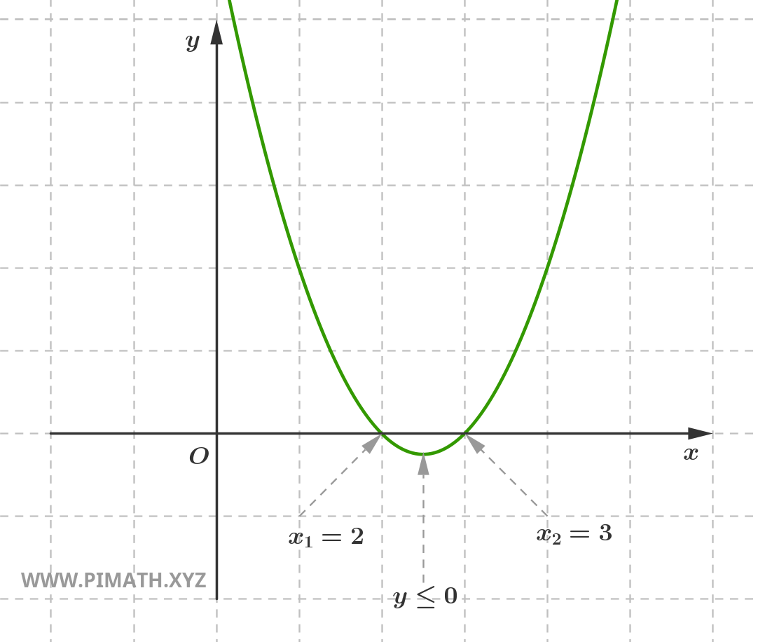
therefore \( x_1 = 2 \) and \( x_2 = 3 \).
Since the coefficient of the term \( x^2 \) is positive, the parabola has its concavity facing upward and the inequality will be satisfied in the interval between the two solutions.
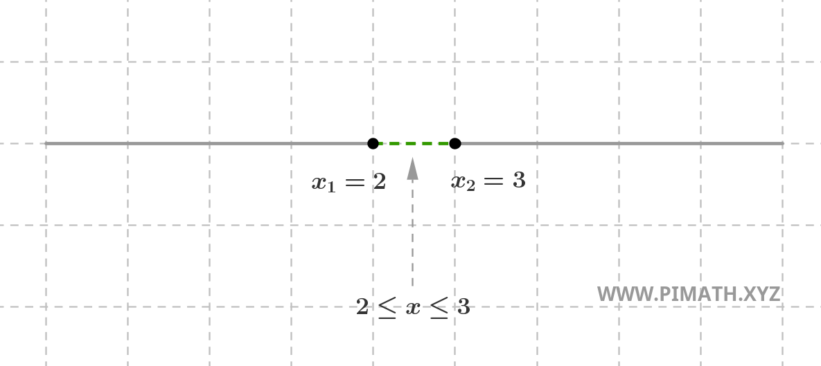
The solutions \( 2 \leq x \leq 3 \) can be graphically represented as follows:
Usually, to avoid drawing the parabola each time, we prefer to represent the solutions on a line, distinguishing positive values with a continuous line and negative values with a dashed line. For example, the solutions of the previous inequality are represented in this way:
Attention to the inclusion of solutions: If we are studying a strict inequality (\( < \) or \( > \)), the roots of the associated equation must be excluded, and this is represented with empty circles in the graphical representation. If instead the inequality is non-strict (\( \leq \) or \( \geq \)), the roots are included and are indicated with filled circles.
Exercise 2. Solve the second-degree inequality \( 2x^2 - 4x - 6 > 0 \)
Solution. We calculate the discriminant \( \Delta = b^2 - 4ac \)
For this equation, \( a = 2 \), \( b = -4 \), and \( c = -6 \). Substituting these values in the formula:
\[ \Delta = (-4)^2 - 4(2)(-6) = 16 + 48 = 64 \]
Since \( \Delta > 0 \), the equation has two distinct real solutions.
The quadratic formula for the associated equation is:
\[ x_{1,2} = \frac{-b \pm \sqrt{\Delta}}{2a} \]
Substituting \( b = -4 \), \( \Delta = 64 \), and \( a = 2 \) in the formula:
\[ x_{1,2} = \frac{4 \pm \sqrt{64}}{2 \times 2} = \frac{4 \pm 8}{4} \]
The first solution is \( x_1 = \displaystyle \frac{4 - 8}{4} = \displaystyle \frac{-4}{4} = -1 \), the second solution is instead \( x_2 = \displaystyle \frac{4 + 8}{4} = \displaystyle \frac{12}{4} = 3 \).
The solutions of the equation are therefore:
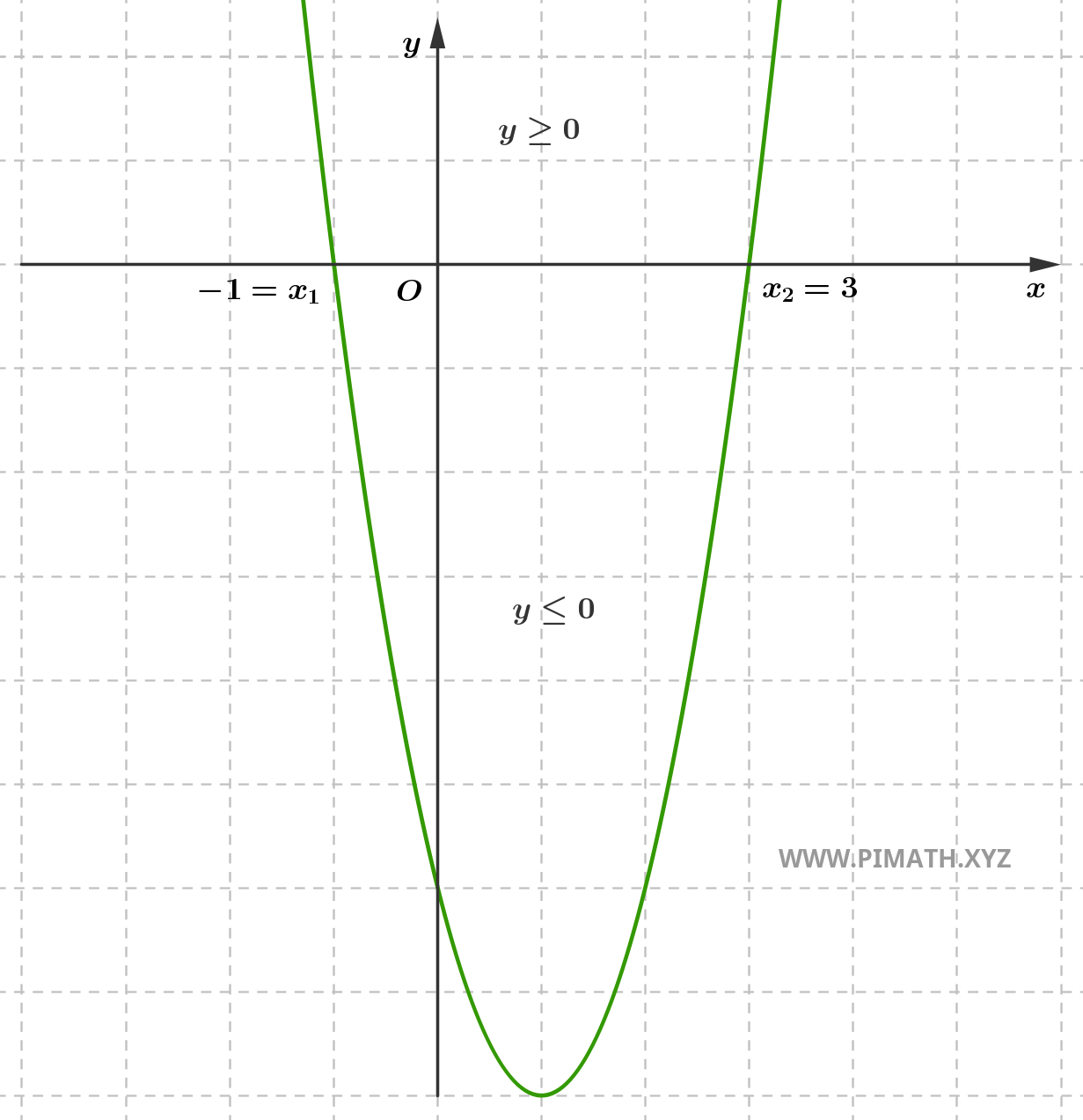
\[ x_1 = -1 \quad \text{and} \quad x_2 = 3 \]
Note that the quadratic coefficient is greater than zero and the inequality asks for the solutions for which we have \( ax^2+bx+c > 0 \), therefore the positive solutions are found "outside the interval", that is \( x < -1 \) or \( x > 3 \), as shown in the graph:
Or:
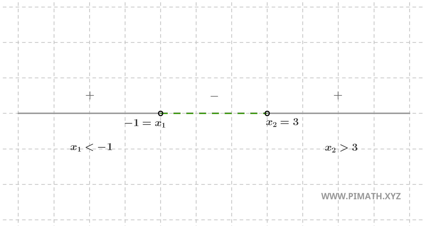
Observe, finally, that the circles are not filled since we are excluding the points \( x = -1 \) and \( x = 3 \).
Exercise 3. Solve the second-degree inequality \( 2x^2+x+1 \leq 0 \).
Solution. The inequality is already presented in canonical form.
We calculate the discriminant:
\[ \Delta = b^2 - 4ac \]
Substituting \( a = 2 \), \( b = 1 \), \( c = 1 \):
\[ \Delta = (1)^2 - 4(2)(1) = 1 - 8 = -7 \]
Since the discriminant is negative, the associated equation \( 2x^2+x+1 = 0 \) has no real solutions.
Furthermore, since the coefficient of the quadratic term is positive (\( a = 2 > 0 \)), the parabola has its concavity facing upward, which means that its value is always positive for any value of \( x \).
For an inequality in the form \( 2x^2+x+1 \leq 0 \) with \( a > 0 \) and negative discriminant, the inequality has no solutions, since the function is always positive and can never be less than or equal to zero.
Therefore, the solution is the empty set. The graph of the function is:
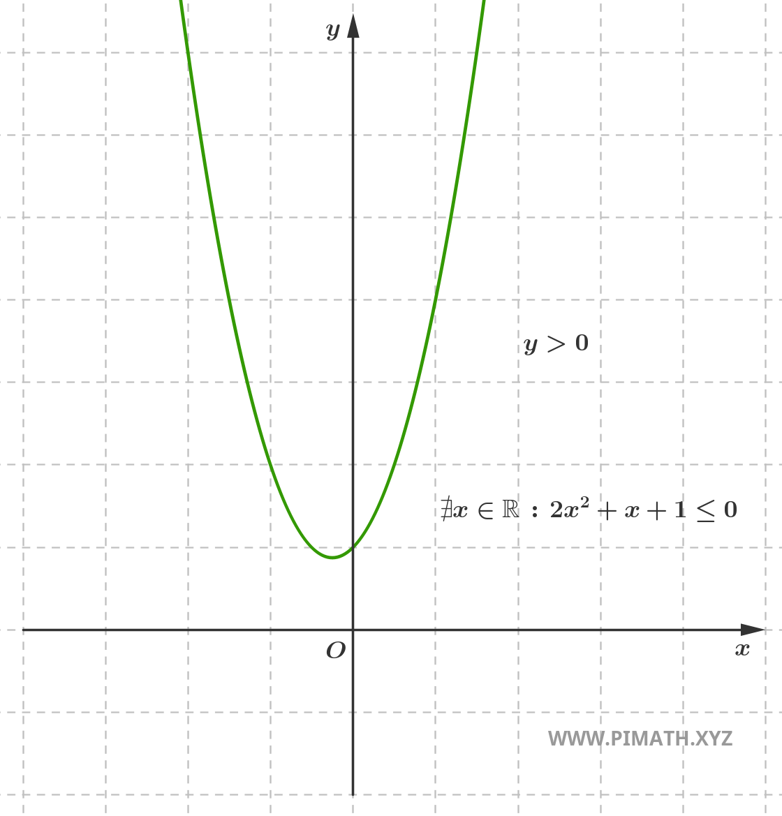
As can be observed, the parabola is always above the \( x \) axis, so there are no values of \( x \) that satisfy the inequality \( 2x^2+x+1 \leq 0 \).