

Sequences provide an orderly and rigorous way to study the behavior of quantities that depend on a natural-number index.
Intuitively, a sequence is an infinite list of numbers:
\[ a_1,\ a_2,\ a_3,\ \ldots,\ a_n,\ \ldots \]
In mathematics, however, a sequence is more than a list written out in order. It is a function defined on the set of natural numbers—a rule that assigns to each natural-number index \(n\) a real number \(a_n\).
This point is essential: to study a sequence is to study how the term \(a_n\) changes as \(n\) grows, and above all to determine whether its terms approach some value, remain bounded, oscillate, grow without bound, or display no regular pattern at all.
Sequences underlie some of the central notions of analysis, such as the limit, convergence, divergence, the completeness of the real numbers, numerical series, and many fundamental properties of functions.
In the following sections, we introduce sequences rigorously, starting from the formal definition and then moving on to their main properties and examples. The goal is to build a solid foundation for the later study of limits of sequences and of the fundamental results of mathematical analysis.
Contents
- Definition of a sequence
- Notation for a sequence
- The general term of a sequence
- Sequences defined explicitly
- Sequences defined by recursion
- Basic examples of sequences
- Constant sequences
- Increasing and decreasing sequences
- Monotonic sequences
- Sequences bounded above and below
- Bounded sequences
- Positive, negative, and alternating sequences
- Arithmetic sequences
- Geometric sequences
- The graph of a sequence
- Sequences versus real functions of a real variable
- Subsequences
- First properties of sequences
- Common mistakes about sequences
Definition of a sequence
A sequence is a function defined on the set of natural numbers.
More precisely, a real sequence is a function
\[ a:\mathbb N\to\mathbb R. \]
This means that to each natural number \(n\in\mathbb N\) the function \(a\) assigns one and only one real number, written
\[ a(n). \]
When working with sequences, however, one almost always uses subscript notation. Instead of writing \(a(n)\), one writes
\[ a_n. \]
The number \(a_n\) is called the \(n\)th term of the sequence.
A real sequence can therefore be viewed as an infinite, ordered list of real numbers:
\[ a_1,\ a_2,\ a_3,\ \ldots,\ a_n,\ \ldots \]
Care is needed, though: this list is not merely a set of numbers. The order of the terms is an essential part of the sequence.
For instance, the two sequences
\[ 1,\ 2,\ 3,\ 4,\ldots \]
and
\[ 2,\ 1,\ 4,\ 3,\ldots \]
are not the same sequence, even though they may take the same values. Indeed, the first term of the first sequence is \(1\), whereas the first term of the second is \(2\).
In general, then, a sequence is not determined solely by the values it takes, but also by the way those values are matched with the natural-number indices.
If \(a:\mathbb N\to\mathbb R\) is a sequence, it is often denoted by one of the following notations:
\[ (a_n)_{n\in\mathbb N}, \qquad (a_n), \qquad \{a_n\}_{n\in\mathbb N}. \]
We will mainly use the notation
\[ (a_n)_{n\in\mathbb N}. \]
This notation emphasizes that the sequence is the whole object made up of all the terms \(a_n\), as \(n\) ranges over the natural numbers.
It is important to distinguish between the sequence and its general term. The sequence is the entire function
\[ (a_n)_{n\in\mathbb N}, \]
whereas \(a_n\) is merely the term corresponding to the index \(n\).
For example, if
\[ a_n=\frac1n, \]
then the sequence is
\[ 1,\ \frac12,\ \frac13,\ \frac14,\ldots \]
and the general term is
\[ a_n=\frac1n. \]
To sum up, a real sequence is a function that assigns a real number to each natural-number index. Subscript notation lets us study how the terms behave as \(n\) grows, which is the starting point for the theory of limits of sequences.
Notation for a sequence
Having defined a sequence as a function on the natural numbers, we now fix a few notational conventions.
A sequence is usually denoted by
\[ (a_n)_{n\in\mathbb N}. \]
This expression means that we are considering all the terms \(a_n\) as the index \(n\) ranges over the set \(\mathbb N\).
In many texts, though, the set of natural numbers can be defined in two different ways:
\[ \mathbb N=\{0,1,2,3,\ldots\} \]
or
\[ \mathbb N=\{1,2,3,\ldots\}. \]
For this reason, when working with sequences it is often necessary to specify the index at which the sequence begins.
If the sequence starts at \(0\), one writes
\[ (a_n)_{n\ge 0}. \]
In this case the terms are
\[ a_0,\ a_1,\ a_2,\ a_3,\ldots \]
If instead the sequence starts at \(1\), one writes
\[ (a_n)_{n\ge 1}. \]
In this case the terms are
\[ a_1,\ a_2,\ a_3,\ldots \]
Both conventions are correct. The choice of the starting index does not change the nature of the sequence, but it can change the way its terms are written.
For example, the sequence
\[ a_n=\frac{1}{n} \]
cannot be considered for \(n=0\), since \(\displaystyle \frac{1}{0}\) is undefined. Here it is natural to write
\[ (a_n)_{n\ge 1}. \]
The sequence
\[ b_n=\frac{1}{n+1}, \]
on the other hand, can be considered for \(n\ge 0\). In that case one obtains
\[ b_0=1,\qquad b_1=\frac12,\qquad b_2=\frac13,\qquad b_3=\frac14,\ldots \]
The two sequences
\[ (a_n)_{n\ge 1}, \qquad (b_n)_{n\ge 0} \]
take the same values in the same order, but they are indexed differently.
In general, when no ambiguity arises, one may simply write
\[ (a_n). \]
In definitions and proofs, however, stating the index set clearly prevents errors and ambiguity.
We will mainly use sequences indexed by \(n\ge 1\), unless stated otherwise.
The general term of a sequence
The general term of a sequence is the expression that describes the term \(a_n\) as a function of the index \(n\).
For example, if
\[ a_n=\frac{n+1}{n}, \]
then the general term of the sequence is
\[ \frac{n+1}{n}. \]
Substituting the values \(1,2,3,4,\ldots\) for \(n\), we obtain the terms of the sequence:
\[ a_1=2,\qquad a_2=\frac32,\qquad a_3=\frac43,\qquad a_4=\frac54,\ldots \]
Hence the sequence is
\[ 2,\ \frac32,\ \frac43,\ \frac54,\ldots \]
The general term lets us compute any term of the sequence, provided the index in question belongs to the index set on which the sequence is defined.
This caveat matters. Writing down a formula is not enough: one must also establish for which values of \(n\) that formula makes sense.
For example, the expression
\[ a_n=\frac{1}{n-3} \]
does not define a sequence for all indices \(n\ge 1\), because the denominator vanishes when \(n=3\).
To obtain a real sequence, we must therefore restrict the index set, for instance by requiring
\[ n\ge 4. \]
In that case we obtain the sequence
\[ a_4=1,\qquad a_5=\frac12,\qquad a_6=\frac13,\qquad a_7=\frac14,\ldots \]
A common mistake is to confuse the general term with the sequence itself. The general term \(a_n\) is a single term that varies with \(n\); the sequence \((a_n)\), by contrast, is the whole object made up of all the terms.
For example, in the sequence
\[ a_n=n^2+1, \]
the general term is \(n^2+1\), while the first terms are
\[ 2,\ 5,\ 10,\ 17,\ 26,\ldots \]
Knowing the general term is often the simplest way to study the properties of a sequence: monotonicity, boundedness, the sign of the terms, and behavior for large values of the index.
Sequences defined explicitly
A sequence is said to be defined explicitly when its general term is given directly by a formula in terms of the index \(n\).
In other words, a sequence is defined explicitly when we can write
\[ a_n=f(n), \]
where \(f\) is some expression depending on \(n\).
For example, the sequence
\[ a_n=2n+1 \]
is defined explicitly. Indeed, substituting the values \(1,2,3,\ldots\) for \(n\), we obtain its terms directly:
\[ a_1=3,\qquad a_2=5,\qquad a_3=7,\qquad a_4=9,\ldots \]
Hence the sequence is
\[ 3,\ 5,\ 7,\ 9,\ldots \]
The sequence
\[ b_n=\frac{n}{n+1} \]
is also defined explicitly. Its first terms are
\[ b_1=\frac12,\qquad b_2=\frac23,\qquad b_3=\frac34,\qquad b_4=\frac45,\ldots \]
Here the formula lets us compute any term of the sequence at once.
For example, the hundredth term is
\[ b_{100}=\frac{100}{101}. \]
This is an important feature of explicitly defined sequences: to find a term, there is no need to know the preceding ones.
Consider now the sequence
\[ c_n=(-1)^n. \]
For \(n\ge 1\), its first terms are
\[ c_1=-1,\qquad c_2=1,\qquad c_3=-1,\qquad c_4=1,\ldots \]
Thus the sequence is
\[ -1,\ 1,\ -1,\ 1,\ldots \]
This example shows that an explicit formula can also describe sequences that are neither increasing nor decreasing, but oscillating.
In general, explicitly defined sequences are especially convenient, because they let us study the properties of the sequence directly from the formula for the general term.
For example, from the formula
\[ a_n=\frac{1}{n} \]
one sees that the terms are positive and become smaller and smaller as \(n\) grows:
\[ 1,\ \frac12,\ \frac13,\ \frac14,\ldots \]
From the formula
\[ a_n=n^2, \]
on the other hand, one sees that the terms grow without bound:
\[ 1,\ 4,\ 9,\ 16,\ldots \]
One must remember, however, that an explicit formula defines a real sequence only if it makes sense for all the indices under consideration.
For example, the formula
\[ a_n=\sqrt{n-5} \]
does not define a real sequence for all indices \(n\ge 1\), because for \(n=1,2,3,4\) the quantity \(n-5\) is negative.
To obtain a real sequence, we may consider it from \(n=5\) onward:
\[ (a_n)_{n\ge 5}, \qquad a_n=\sqrt{n-5}. \]
In this way all the terms are real numbers:
\[ a_5=0,\qquad a_6=1,\qquad a_7=\sqrt2,\qquad a_8=\sqrt3,\ldots \]
Thus, whenever a sequence is defined explicitly, two things must always be checked:
- the formula for the general term;
- the set of indices for which the formula is defined.
Once these two elements are fixed, the sequence is completely determined.
Sequences defined by recursion
A sequence is said to be defined by recursion when its terms are not given directly by an explicit formula in terms of \(n\), but are instead obtained from one or more preceding terms.
In this case, defining the sequence requires more than stating a relation among the terms: at least one initial term must also be specified.
For example, consider the sequence defined by
\[ a_1=2, \qquad a_{n+1}=a_n+3 \quad \text{for all } n\ge 1. \]
The first term is \(a_1=2\). The recurrence relation says that each successive term is obtained by adding \(3\) to the preceding one.
We therefore obtain
\[ a_2=a_1+3=5, \]
\[ a_3=a_2+3=8, \]
\[ a_4=a_3+3=11. \]
Hence the sequence is
\[ 2,\ 5,\ 8,\ 11,\ldots \]
In a recursively defined sequence, computing a term often requires knowing the terms that come before it.
Consider a second example:
\[ b_1=1, \qquad b_{n+1}=2b_n \quad \text{for all } n\ge 1. \]
Here each successive term is obtained by multiplying the preceding one by \(2\):
\[ b_2=2b_1=2, \]
\[ b_3=2b_2=4, \]
\[ b_4=2b_3=8. \]
Hence the sequence is
\[ 1,\ 2,\ 4,\ 8,\ldots \]
A recurrence relation may also depend on more than one preceding term. A fundamental example is the Fibonacci sequence:
\[ F_1=1,\qquad F_2=1, \]
\[ F_{n+2}=F_{n+1}+F_n \quad \text{for all } n\ge 1. \]
Here each term, starting from the third, is the sum of the two preceding terms.
Indeed:
\[ F_3=F_2+F_1=2, \]
\[ F_4=F_3+F_2=3, \]
\[ F_5=F_4+F_3=5, \]
\[ F_6=F_5+F_4=8. \]
The first terms are therefore
\[ 1,\ 1,\ 2,\ 3,\ 5,\ 8,\ldots \]
This example shows that when the recurrence relation involves two preceding terms, two initial terms must be specified. More generally, a recurrence depending on \(k\) preceding terms requires \(k\) initial conditions.
It is worth noting that a recursive definition is not automatically equivalent to a simple explicit formula. Sometimes a closed form for \(a_n\) can be found; other times the recursive description is the most natural way to define the sequence.
For example, the sequence
\[ a_1=2, \qquad a_{n+1}=a_n+3 \]
can also be described explicitly as
\[ a_n=2+3(n-1). \]
Indeed, starting from \(2\), one adds \(3\) to pass from one term to the next; after \(n-1\) steps, \(3\) has been added exactly \(n-1\) times.
In conclusion, a recursively defined sequence is determined by:
- one or more initial terms;
- a rule for constructing the successive terms.
Without the initial conditions, the recurrence relation does not determine a unique sequence.
Basic examples of sequences
Having introduced explicitly defined sequences and recursively defined ones, it is useful to examine some basic examples. These examples occur often in the study of mathematical analysis and help one recognize the most common behaviors of sequences.
The sequence of natural numbers
The sequence
\[ a_n=n \]
has terms
\[ 1,\ 2,\ 3,\ 4,\ldots \]
It is an increasing sequence, and its terms become arbitrarily large as \(n\) grows.
The sequence of reciprocals
The sequence
\[ a_n=\frac1n \]
has terms
\[ 1,\ \frac12,\ \frac13,\ \frac14,\ldots \]
Its terms are positive and become smaller and smaller. This is one of the fundamental examples of a sequence that approaches \(0\).
The sequence of squares
The sequence
\[ a_n=n^2 \]
has terms
\[ 1,\ 4,\ 9,\ 16,\ldots \]
It is an increasing sequence, and its terms grow faster than those of the sequence \(a_n=n\).
The alternating sequence
The sequence
\[ a_n=(-1)^n \]
has terms, for \(n\ge 1\),
\[ -1,\ 1,\ -1,\ 1,\ldots \]
The terms do not approach a single value; instead they oscillate endlessly between \(-1\) and \(1\).
The harmonic sequence
The sequence
\[ a_n=1+\frac12+\frac13+\cdots+\frac1n \]
is the sequence of partial sums of the harmonic series.
Its first terms are
\[ a_1=1, \qquad a_2=1+\frac12=\frac32, \]
\[ a_3=1+\frac12+\frac13=\frac{11}{6}, \qquad a_4=1+\frac12+\frac13+\frac14=\frac{25}{12}. \]
This sequence is increasing. Even though the individual summands \(\frac1n\) become smaller and smaller, the partial sums keep growing.
A basic geometric sequence
The sequence
\[ a_n=2^n \]
has terms, for \(n\ge 1\),
\[ 2,\ 4,\ 8,\ 16,\ldots \]
Each term is obtained from the preceding one by multiplying by \(2\). For this reason it is an example of a geometric sequence.
A decreasing geometric sequence
The sequence
\[ a_n=\left(\frac12\right)^n \]
has terms, for \(n\ge 1\),
\[ \frac12,\ \frac14,\ \frac18,\ \frac1{16},\ldots \]
Each term is obtained from the preceding one by multiplying by \(\frac12\). The terms are positive and gradually approach \(0\).
A sequence defined by a ratio
The sequence
\[ a_n=\frac{n}{n+1} \]
has terms
\[ \frac12,\ \frac23,\ \frac34,\ \frac45,\ldots \]
All the terms are less than \(1\), but they get closer and closer to \(1\).
Indeed, we can write
\[ \frac{n}{n+1}=1-\frac{1}{n+1}. \]
This form shows clearly that the distance between \(a_n\) and \(1\) equals \(\displaystyle \frac{1}{n+1}\), which becomes smaller and smaller as \(n\) grows.
A sequence with alternating sign and decreasing magnitude
The sequence
\[ a_n=\frac{(-1)^n}{n} \]
has terms
\[ -1,\ \frac12,\ -\frac13,\ \frac14,\ldots \]
The terms change sign at each step, but their magnitude becomes smaller and smaller.
In particular, both the positive and the negative terms approach \(0\).
These examples show that sequences can behave in very different ways: they may increase, decrease, oscillate, remain bounded, approach a number, or grow arbitrarily large.
Constant sequences
A sequence is said to be constant if all its terms equal one and the same real number.
More precisely, a real sequence \((a_n)_{n\ge 1}\) is constant if there exists a real number \(c\) such that
\[ a_n=c \quad \text{for all } n\ge 1. \]
In this case the sequence is
\[ c,\ c,\ c,\ c,\ldots \]
For example, the sequence defined by
\[ a_n=5 \quad \text{for all } n\ge 1 \]
is constant, since each of its terms equals \(5\):
\[ 5,\ 5,\ 5,\ 5,\ldots \]
The sequence
\[ b_n=-2 \quad \text{for all } n\ge 1 \]
is also constant:
\[ -2,\ -2,\ -2,\ -2,\ldots \]
Constant sequences are the simplest examples of sequences. They neither increase nor decrease in the strict sense, and they do not oscillate: all the terms coincide.
From the standpoint of monotonicity, a constant sequence is both increasing and decreasing, in the non-strict sense:
\[ a_n\le a_{n+1} \quad \text{for all } n\ge 1, \]
and
\[ a_n\ge a_{n+1} \quad \text{for all } n\ge 1. \]
Indeed, if \(a_n=c\) for all \(n\), then
\[ a_n=a_{n+1}=c. \]
Hence both \(a_n\le a_{n+1}\) and \(a_n\ge a_{n+1}\) hold simultaneously.
A constant sequence is also bounded. Indeed, if \(a_n=c\) for all \(n\), then all its terms coincide with \(c\), so they certainly lie, for example, between \(c-1\) and \(c+1\):
\[ c-1\le a_n\le c+1 \quad \text{for all } n\ge 1. \]
In fact, the least upper bound of the set of values taken by the sequence is \(c\), and the greatest lower bound is \(c\) as well. Indeed, the set of values taken is simply
\[ \{c\}. \]
Hence
\[ \sup\{a_n:n\ge 1\}=c, \qquad \inf\{a_n:n\ge 1\}=c. \]
Constant sequences are also important because they represent the simplest model of a sequence that always stays equal to a fixed value.
Increasing and decreasing sequences
A sequence can be studied by comparing each term with the next. This makes it possible to tell whether the terms increase, decrease, or follow no regular pattern.
A real sequence \((a_n)_{n\ge 1}\) is called increasing if
\[ a_n\le a_{n+1} \quad \text{for all } n\ge 1. \]
In other words, each term is less than or equal to the next.
It is called strictly increasing if
\[ a_n<a_{n+1} \quad \text{for all } n\ge 1. \]
In this case each term is strictly less than the next.
For example, the sequence
\[ a_n=n \]
is strictly increasing, since
\[ a_{n+1}=n+1>n=a_n \quad \text{for all } n\ge 1. \]
Hence its terms are
\[ 1,\ 2,\ 3,\ 4,\ldots \]
and they increase at each step.
A real sequence \((a_n)_{n\ge 1}\) is called decreasing if
\[ a_n\ge a_{n+1} \quad \text{for all } n\ge 1. \]
In other words, each term is greater than or equal to the next.
It is called strictly decreasing if
\[ a_n>a_{n+1} \quad \text{for all } n\ge 1. \]
For example, the sequence
\[ b_n=\frac1n \]
is strictly decreasing, since
\[ b_{n+1}=\frac{1}{n+1}<\frac1n=b_n \quad \text{for all } n\ge 1. \]
Indeed, its terms are
\[ 1,\ \frac12,\ \frac13,\ \frac14,\ldots \]
and they become smaller and smaller.
Not every sequence is increasing or decreasing. For example, the sequence
\[ c_n=(-1)^n \]
has terms
\[ -1,\ 1,\ -1,\ 1,\ldots \]
and so it is neither increasing nor decreasing.
Indeed, from \(c_1=-1\) to \(c_2=1\) the sequence increases, while from \(c_2=1\) to \(c_3=-1\) it decreases.
To check whether a sequence is increasing or decreasing, a widely used method is to study the sign of the difference
\[ a_{n+1}-a_n. \]
If
\[ a_{n+1}-a_n\ge 0 \quad \text{for all } n\ge 1, \]
then the sequence is increasing.
If instead
\[ a_{n+1}-a_n\le 0 \quad \text{for all } n\ge 1, \]
then the sequence is decreasing.
For example, consider
\[ a_n=n^2. \]
We compute:
\[ a_{n+1}-a_n=(n+1)^2-n^2. \]
Expanding,
\[ (n+1)^2-n^2=n^2+2n+1-n^2=2n+1. \]
Since
\[ 2n+1>0 \quad \text{for all } n\ge 1, \]
the sequence \((n^2)_{n\ge 1}\) is strictly increasing.
Another method, useful when the terms are positive, is to study the ratio
\[ \frac{a_{n+1}}{a_n}. \]
If \(a_n>0\) for all \(n\) and
\[ \frac{a_{n+1}}{a_n}\ge 1 \quad \text{for all } n\ge 1, \]
then the sequence is increasing.
If instead \(a_n>0\) for all \(n\) and
\[ \frac{a_{n+1}}{a_n}\le 1 \quad \text{for all } n\ge 1, \]
then the sequence is decreasing.
For example, consider
\[ a_n=\left(\frac12\right)^n. \]
Since \(a_n>0\) for all \(n\ge 1\), we can study the ratio:
\[ \frac{a_{n+1}}{a_n} = \frac{\left(\frac12\right)^{n+1}}{\left(\frac12\right)^n} = \frac12. \]
Because
\[ \frac12<1, \]
the sequence is strictly decreasing.
It is important to remember that an increasing sequence need not grow without bound. For example,
\[ a_n=\frac{n}{n+1} \]
is increasing, yet all its terms are less than \(1\):
\[ \frac12,\ \frac23,\ \frac34,\ \frac45,\ldots \]
Likewise, a decreasing sequence need not become arbitrarily negative. For example,
\[ b_n=\frac1n \]
is decreasing, yet all its terms are positive.
Monotonic sequences
A sequence is called monotonic if it always keeps the same direction of variation: either it never decreases, or it never increases.
More precisely, a real sequence \((a_n)_{n\ge 1}\) is called monotonic if it is increasing or decreasing.
Thus a sequence is monotonic if one of the following two conditions holds:
\[ a_n\le a_{n+1} \quad \text{for all } n\ge 1, \]
or
\[ a_n\ge a_{n+1} \quad \text{for all } n\ge 1. \]
In the first case the sequence is increasing; in the second it is decreasing.
If instead
\[ a_n<a_{n+1} \quad \text{for all } n\ge 1, \]
the sequence is strictly increasing. If
\[ a_n>a_{n+1} \quad \text{for all } n\ge 1, \]
the sequence is strictly decreasing.
A sequence that is strictly increasing or strictly decreasing is called strictly monotonic.
For example, the sequence
\[ a_n=3n+1 \]
is strictly increasing, since
\[ a_{n+1}=3(n+1)+1=3n+4 \]
and hence
\[ a_{n+1}-a_n=(3n+4)-(3n+1)=3>0 \quad \text{for all } n\ge 1. \]
Therefore
\[ a_n<a_{n+1} \quad \text{for all } n\ge 1, \]
and the sequence is strictly increasing.
Consider instead the sequence
\[ b_n=\frac{1}{n+2}. \]
Its first terms are
\[ \frac13,\ \frac14,\ \frac15,\ \frac16,\ldots \]
Since the denominator increases as \(n\) grows, the terms become smaller.
Indeed
\[ b_{n+1}=\frac{1}{n+3} \]
and, since
\[ n+3>n+2 \quad \text{for all } n\ge 1, \]
we have
\[ \frac{1}{n+3}<\frac{1}{n+2}. \]
Hence
\[ b_{n+1}<b_n \quad \text{for all } n\ge 1, \]
that is, the sequence is strictly decreasing.
Not every sequence is monotonic. For example, the sequence
\[ c_n=(-1)^n \]
is not monotonic, because its terms are
\[ -1,\ 1,\ -1,\ 1,\ldots \]
and so the sequence first increases, then decreases, then increases again.
Indeed
\[ c_1=-1<1=c_2, \]
but
\[ c_2=1>-1=c_3. \]
Hence it is neither increasing nor decreasing.
Monotonicity is an important property because it imposes a global order on the terms of the sequence. If a sequence is increasing, no later term can drop below the earlier ones; if it is decreasing, no later term can rise above the earlier ones.
For example, if \((a_n)\) is increasing, then
\[ a_1\le a_2\le a_3\le \cdots \le a_n\le a_{n+1}\le \cdots. \]
If instead \((a_n)\) is decreasing, then
\[ a_1\ge a_2\ge a_3\ge \cdots \ge a_n\ge a_{n+1}\ge \cdots. \]
This ordered structure makes monotonic sequences especially important in the study of limits. Indeed, a sequence that is monotonic and bounded always has a real limit; this result, known as the monotone convergence theorem, will be one of the central points in the later study of sequences.
Sequences bounded above and below
A sequence can also be studied in terms of the values its terms can take. In particular, it is important to determine whether the terms always stay below a certain number or always above a certain number.
Let \((a_n)_{n\ge 1}\) be a real sequence. We say that \((a_n)\) is bounded above if there exists a real number \(M\) such that
\[ a_n\le M \quad \text{for all } n\ge 1. \]
The number \(M\) is called an upper bound of the sequence.
Similarly, we say that \((a_n)\) is bounded below if there exists a real number \(m\) such that
\[ m\le a_n \quad \text{for all } n\ge 1. \]
The number \(m\) is called a lower bound of the sequence.
For example, the sequence
\[ a_n=\frac{n}{n+1} \]
is bounded above. Indeed
\[ \frac{n}{n+1}<1 \quad \text{for all } n\ge 1. \]
Hence \(1\) is an upper bound of the sequence.
Note, however, that \(1\) is not the only upper bound. The numbers \(2\), \(10\), \(100\) are upper bounds as well, since all the terms of the sequence are less than \(1\), and therefore certainly less than \(2\), \(10\), \(100\) too.
In general, if \(M\) is an upper bound of a sequence, then every number greater than \(M\) is again an upper bound.
The same sequence is also bounded below. Indeed, for every \(n\ge 1\),
\[ \frac{n}{n+1}>0. \]
Hence \(0\) is a lower bound of the sequence.
Here too the lower bound is not unique: every number less than or equal to \(0\) is a lower bound.
Consider now the sequence
\[ b_n=n. \]
It is bounded below, since
\[ 1\le n \quad \text{for all } n\ge 1. \]
Hence \(1\) is a lower bound.
The sequence is not bounded above, however. Indeed, there is no real number \(M\) such that
\[ n\le M \quad \text{for all } n\ge 1. \]
Whatever real number \(M\) we choose, there is always a natural-number index \(n\) such that
\[ n>M. \]
Hence the terms of the sequence exceed any fixed threshold.
Consider instead the sequence
\[ c_n=-n. \]
It is bounded above, since
\[ -n\le -1 \quad \text{for all } n\ge 1. \]
Hence \(-1\) is an upper bound.
It is not bounded below, however: its terms become more and more negative and drop below any fixed real number.
In symbols, for every \(m\in\mathbb R\) there is a natural-number index \(n\) such that
\[ -n<m. \]
Hence there is no real lower bound for the sequence \((-n)_{n\ge 1}\).
It is important to distinguish between a sequence being bounded above or below and a sequence being increasing or decreasing.
For example, the sequence
\[ a_n=\frac{n}{n+1} \]
is increasing, yet it is bounded above by \(1\). Thus an increasing sequence need not grow without bound.
Likewise, the sequence
\[ b_n=\frac1n \]
is decreasing, yet it is bounded below by \(0\). Thus a decreasing sequence need not become arbitrarily negative.
From the set-theoretic standpoint, saying that a sequence is bounded above means that its set of values
\[ \{a_n:n\ge 1\} \]
is a subset of \(\mathbb R\) that is bounded above.
Likewise, saying that a sequence is bounded below means that the set
\[ \{a_n:n\ge 1\} \]
is bounded below.
This observation lets us connect the study of sequences with the theory of the supremum and the infimum.
If a sequence is bounded above, its set of values has a supremum:
\[ \sup\{a_n:n\ge 1\}. \]
If a sequence is bounded below, its set of values has an infimum:
\[ \inf\{a_n:n\ge 1\}. \]
For example, for the sequence
\[ a_n=\frac{n}{n+1} \]
the set of values is
\[ \left\{\frac12,\frac23,\frac34,\frac45,\ldots\right\}. \]
It is bounded above, and its supremum is \(1\), even though \(1\) is not a term of the sequence.
Indeed
\[ \frac{n}{n+1}<1 \quad \text{for all } n\ge 1, \]
but the terms get closer and closer to \(1\).
Bounded sequences
A sequence is called bounded if it is bounded both above and below.
More precisely, a real sequence \((a_n)_{n\ge 1}\) is bounded if there exist two real numbers \(m\) and \(M\) such that
\[ m\le a_n\le M \quad \text{for all } n\ge 1. \]
The number \(m\) is a lower bound of the sequence, while \(M\) is an upper bound.
Equivalently, a sequence is bounded if all its terms lie in a closed, bounded interval:
\[ a_n\in [m,M] \quad \text{for all } n\ge 1. \]
For example, the sequence
\[ a_n=\frac{1}{n} \]
is bounded. Indeed, for every \(n\ge 1\) we have
\[ 0<\frac1n\le 1. \]
Hence all the terms of the sequence lie between \(0\) and \(1\):
\[ 0\le a_n\le 1 \quad \text{for all } n\ge 1. \]
Note that \(0\) is a lower bound but is not a term of the sequence. Indeed, there is no \(n\ge 1\) such that
\[ \frac1n=0. \]
This shows that a lower bound or an upper bound need not be attained by the sequence.
The sequence
\[ b_n=(-1)^n \]
is also bounded. Indeed, its terms are only \(-1\) and \(1\):
\[ -1,\ 1,\ -1,\ 1,\ldots \]
Hence
\[ -1\le b_n\le 1 \quad \text{for all } n\ge 1. \]
In this case both the lower bound \(-1\) and the upper bound \(1\) are values that the sequence actually attains.
The sequence
\[ c_n=n, \]
on the other hand, is not bounded. Indeed, it is bounded below, since
\[ 1\le n \quad \text{for all } n\ge 1, \]
but it is not bounded above.
For every \(M\in\mathbb R\), one can choose a natural-number index \(n\) such that
\[ n>M. \]
Hence there is no real number \(M\) that can bound all the terms of the sequence from above.
Likewise, the sequence
\[ d_n=-n \]
is not bounded, because it is bounded above but not below.
Another widely used characterization of boundedness is the one in terms of the absolute value.
A real sequence \((a_n)_{n\ge 1}\) is bounded if and only if there exists a real number \(K>0\) such that
\[ |a_n|\le K \quad \text{for all } n\ge 1. \]
This condition means that all the terms of the sequence belong to the interval
\[ [-K,K]. \]
Indeed, from the inequality
\[ |a_n|\le K \]
it follows that
\[ -K\le a_n\le K \quad \text{for all } n\ge 1. \]
Conversely, if there exist \(m,M\in\mathbb R\) such that
\[ m\le a_n\le M \quad \text{for all } n\ge 1, \]
then it suffices to choose
\[ K=\max\{|m|,|M|\}. \]
In this way one obtains
\[ |a_n|\le K \quad \text{for all } n\ge 1. \]
This form is often more convenient in proofs, because it captures both the upper and the lower control of the terms in a single inequality.
For example, the sequence
\[ a_n=\frac{(-1)^n}{n} \]
is bounded, since
\[ |a_n| = \left|\frac{(-1)^n}{n}\right| = \frac1n \le 1 \quad \text{for all } n\ge 1. \]
Hence we can choose \(K=1\) and conclude that
\[ |a_n|\le 1 \quad \text{for all } n\ge 1. \]
Boundedness is an essential property in the study of sequences. By itself it does not guarantee the existence of a limit: for example, \((-1)^n\) is bounded but does not approach a single value.
Combined with other properties, such as monotonicity, however, it becomes extremely powerful. In particular, every monotonic and bounded sequence converges to a real number.
Positive, negative, and alternating sequences
Another important aspect in the study of a sequence is the sign of its terms. In particular, it can be useful to determine whether the terms are always positive, always negative, or change sign as the index varies.
A real sequence \((a_n)_{n\ge 1}\) is called positive if
\[ a_n\ge 0 \quad \text{for all } n\ge 1. \]
If instead
\[ a_n>0 \quad \text{for all } n\ge 1, \]
the sequence is called strictly positive.
For example, the sequence
\[ a_n=\frac1n \]
is strictly positive, since
\[ \frac1n>0 \quad \text{for all } n\ge 1. \]
A real sequence \((a_n)_{n\ge 1}\) is called negative if
\[ a_n\le 0 \quad \text{for all } n\ge 1. \]
If instead
\[ a_n<0 \quad \text{for all } n\ge 1, \]
the sequence is called strictly negative.
For example, the sequence
\[ b_n=-n \]
is strictly negative, since
\[ -n<0 \quad \text{for all } n\ge 1. \]
A sequence may also contain both positive and negative terms. A particularly important case is that of alternating sequences.
A sequence is called alternating when its terms change sign at each step, passing from positive to negative or from negative to positive.
The fundamental example is
\[ a_n=(-1)^n. \]
For \(n\ge 1\), its terms are
\[ -1,\ 1,\ -1,\ 1,\ldots \]
Indeed, when \(n\) is odd, \((-1)^n=-1\); when \(n\) is even, \((-1)^n=1\).
If instead we consider the sequence
\[ b_n=(-1)^{n+1}, \]
the terms are
\[ 1,\ -1,\ 1,\ -1,\ldots \]
In this case the first term is positive, since
\[ b_1=(-1)^2=1. \]
Powers of \(-1\) are thus a standard tool for building sequences with alternating sign.
For example, the sequence
\[ c_n=\frac{(-1)^n}{n} \]
has terms
\[ -1,\ \frac12,\ -\frac13,\ \frac14,\ldots \]
It changes sign at each step, but the magnitude of the terms decreases.
Indeed
\[ |c_n| = \left|\frac{(-1)^n}{n}\right| = \frac1n. \]
Studying the sign is useful because many properties of sequences depend on whether the terms are positive, negative, or alternating.
For example, when a sequence has positive terms, one can often study monotonicity by means of the ratio
\[ \frac{a_{n+1}}{a_n}. \]
This method requires care: the ratio is especially effective when the terms are strictly positive, since in that case the sign does not reverse the direction of the inequalities.
For alternating sequences, by contrast, monotonicity must be studied more cautiously. For example, the sequence
\[ \frac{(-1)^n}{n} \]
is not monotonic, because its terms keep passing from negative to positive.
The sequence of absolute values
\[ \left|\frac{(-1)^n}{n}\right|=\frac1n, \]
however, is strictly decreasing.
This example reveals an important distinction: a sequence may fail to be monotonic, while the sequence of its absolute values is monotonic.
Arithmetic sequences
An arithmetic sequence is a sequence in which the difference between two consecutive terms is constant.
More precisely, a real sequence \((a_n)_{n\ge 1}\) is arithmetic if there exists a real number \(d\) such that
\[ a_{n+1}-a_n=d \quad \text{for all } n\ge 1. \]
The number \(d\) is called the common difference of the arithmetic sequence.
Equivalently, an arithmetic sequence can be defined by recursion by setting
\[ a_{n+1}=a_n+d \quad \text{for all } n\ge 1. \]
This means that each term is obtained from the preceding one by always adding the same number \(d\).
For example, the sequence
\[ 3,\ 7,\ 11,\ 15,\ldots \]
is arithmetic, since the difference between two consecutive terms is always \(4\):
\[ 7-3=4,\qquad 11-7=4,\qquad 15-11=4. \]
In this case the common difference is
\[ d=4. \]
If the first term is \(a_1\) and the common difference is \(d\), then the general term of the arithmetic sequence is
\[ a_n=a_1+(n-1)d. \]
Indeed, to pass from \(a_1\) to \(a_n\) one must add \(d\) exactly \(n-1\) times:
\[ a_2=a_1+d, \]
\[ a_3=a_1+2d, \]
\[ a_4=a_1+3d, \]
and, in general,
\[ a_n=a_1+(n-1)d. \]
For example, in the sequence
\[ 3,\ 7,\ 11,\ 15,\ldots \]
we have \(a_1=3\) and \(d=4\). Hence
\[ a_n=3+(n-1)4. \]
Simplifying,
\[ a_n=4n-1. \]
Indeed:
\[ a_1=4\cdot 1-1=3, \]
\[ a_2=4\cdot 2-1=7, \]
\[ a_3=4\cdot 3-1=11. \]
The sign of the common difference determines the behavior of the sequence.
- If \(d>0\), the sequence is strictly increasing.
- If \(d=0\), the sequence is constant.
- If \(d<0\), the sequence is strictly decreasing.
For example, the sequence
\[ a_n=2+5(n-1) \]
is strictly increasing, since its common difference is \(d=5>0\).
The sequence
\[ b_n=6 \]
is arithmetic with common difference \(d=0\), so it is constant.
The sequence
\[ c_n=10-3(n-1) \]
is strictly decreasing, since its common difference is \(d=-3<0\).
Arithmetic sequences are thus the simplest model of sequences with linear growth or decay: at each step the change is always the same.
Geometric sequences
A geometric sequence is a sequence in which each term is obtained from the preceding one by always multiplying by the same number.
More precisely, a real sequence \((a_n)_{n\ge 1}\) is geometric if there exists a real number \(q\) such that
\[ a_{n+1}=q\,a_n \quad \text{for all } n\ge 1. \]
The number \(q\) is called the common ratio of the geometric sequence.
If \(a_n\neq 0\) for all \(n\ge 1\), the common ratio can be recovered from the ratio of two consecutive terms:
\[ \frac{a_{n+1}}{a_n}=q \quad \text{for all } n\ge 1. \]
For example, the sequence
\[ 3,\ 6,\ 12,\ 24,\ldots \]
is geometric, since each term is obtained from the preceding one by multiplying by \(2\):
\[ 6=2\cdot 3, \qquad 12=2\cdot 6, \qquad 24=2\cdot 12. \]
In this case the common ratio is
\[ q=2. \]
If the first term is \(a_1\) and the common ratio is \(q\), then the general term of the geometric sequence is
\[ a_n=a_1 q^{\,n-1}. \]
Indeed:
\[ a_2=a_1q, \]
\[ a_3=a_2q=a_1q^2, \]
\[ a_4=a_3q=a_1q^3, \]
and, in general,
\[ a_n=a_1q^{\,n-1}. \]
For example, in the sequence
\[ 3,\ 6,\ 12,\ 24,\ldots \]
we have \(a_1=3\) and \(q=2\). Hence
\[ a_n=3\cdot 2^{n-1}. \]
Indeed:
\[ a_1=3\cdot 2^0=3, \]
\[ a_2=3\cdot 2^1=6, \]
\[ a_3=3\cdot 2^2=12. \]
Consider now the sequence
\[ b_n=\left(\frac12\right)^{n-1}. \]
Its first terms are
\[ 1,\ \frac12,\ \frac14,\ \frac18,\ldots \]
This too is a geometric sequence, with first term \(b_1=1\) and common ratio
\[ q=\frac12. \]
Indeed, each term is obtained from the preceding one by multiplying by \(\displaystyle \frac12\).
The behavior of a geometric sequence depends essentially on the common ratio \(q\).
Suppose, for simplicity, that \(a_1>0\). Then:
- if \(q>1\), the sequence is strictly increasing and its terms become larger and larger;
- if \(q=1\), the sequence is constant;
- if \(0<q<1\), the sequence is strictly decreasing and its terms approach \(0\);
- if \(q=0\), every term from the second one on equals \(0\);
- if \(q<0\), the terms change sign at each step.
For example, the sequence
\[ a_n=2^n \]
is geometric with common ratio \(q=2\). Its terms are
\[ 2,\ 4,\ 8,\ 16,\ldots \]
and they grow rapidly.
The sequence
\[ b_n=\left(\frac13\right)^n, \]
on the other hand, is geometric with common ratio
\[ q=\frac13. \]
Its terms are
\[ \frac13,\ \frac19,\ \frac1{27},\ \frac1{81},\ldots \]
and they become smaller and smaller.
An example with negative common ratio is
\[ c_n=(-2)^n. \]
For \(n\ge 1\), its first terms are
\[ -2,\ 4,\ -8,\ 16,\ldots \]
The sequence is geometric with common ratio \(q=-2\). The terms change sign at each step, and their absolute value grows.
Consider finally the sequence
\[ d_n=\left(-\frac12\right)^n. \]
Its first terms are
\[ -\frac12,\ \frac14,\ -\frac18,\ \frac1{16},\ldots \]
In this case the common ratio is
\[ q=-\frac12. \]
The terms change sign at each step, but their absolute value becomes smaller and smaller.
Geometric sequences are fundamental because they describe processes in which the change is not constant in absolute value, but is proportional to the preceding term. For this reason they arise naturally in many settings: exponential growth, decay, compound interest, and the study of geometric series.
The graph of a sequence
A real sequence \((a_n)_{n\ge 1}\) can be represented graphically in the Cartesian plane by associating with each index \(n\) the corresponding term \(a_n\).
In other words, with the sequence \((a_n)_{n\ge 1}\) we associate the points
\[ (1,a_1),\ (2,a_2),\ (3,a_3),\ldots,\ (n,a_n),\ldots \]
The graph of a sequence is thus the set of points
\[ \{(n,a_n):n\ge 1\}. \]
An important difference from the graph of a real function of a real variable should be noted. A sequence is defined only on the natural-number indices, so its graph is not a continuous curve but a discrete set of points.
For example, consider the sequence
\[ a_n=\frac1n. \]
The first points of its graph are
\[ (1,1),\ \left(2,\frac12\right),\ \left(3,\frac13\right),\ \left(4,\frac14\right),\ldots \]
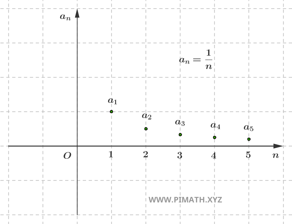
These points descend gradually and approach the horizontal axis, but they do not form a continuous curve.
Likewise, for the sequence
\[ b_n=(-1)^n \]
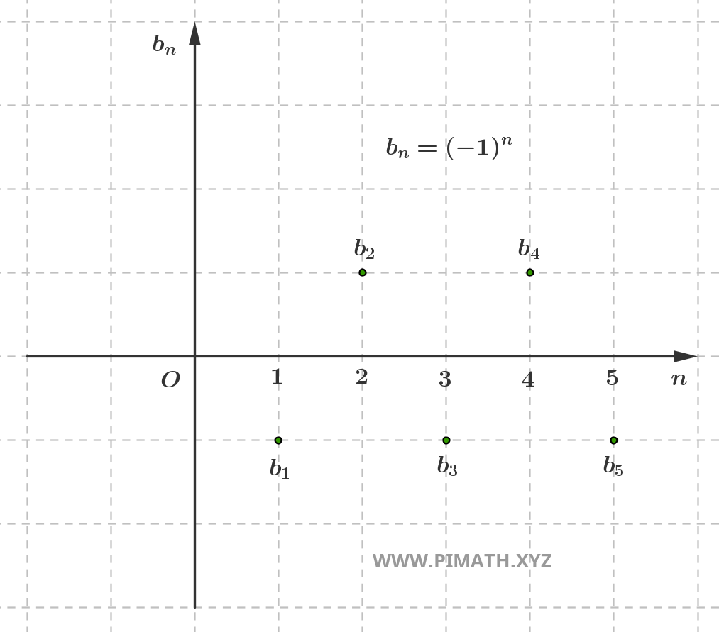
the points of the graph are
\[ (1,-1),\ (2,1),\ (3,-1),\ (4,1),\ldots \]
In this case the points oscillate between the two horizontal lines
\[ y=-1 \qquad \text{and} \qquad y=1. \]
The graphical representation is useful because it lets us visualize some properties of the sequence.
If the points rise as the index grows, the sequence may be increasing. If the points fall, the sequence may be decreasing. If the points stay between two horizontal lines, the sequence may be bounded.
For example, a bounded sequence is represented by points that all stay within a horizontal strip of the plane. Indeed, if there exist \(m,M\in\mathbb R\) such that
\[ m\le a_n\le M \quad \text{for all } n\ge 1, \]
then all the points \((n,a_n)\) lie between the two horizontal lines
\[ y=m \qquad \text{and} \qquad y=M. \]
For example, the sequence
\[ a_n=\frac{n}{n+1} \]
is represented by points lying between \(0\) and \(1\), since
\[ 0<\frac{n}{n+1}<1 \quad \text{for all } n\ge 1. \]
Moreover, the points gradually approach the horizontal line
\[ y=1. \]
It is important, however, not to confuse a picture with a proof. The graph may suggest that a sequence is increasing, bounded, or convergent, but these properties must be verified by means of the definitions or by rigorous criteria.
For example, from the graph of the sequence
\[ a_n=\frac{n}{n+1} \]
one senses that the terms increase and stay below \(1\). To prove it, however, one must check the inequalities.
Indeed
\[ a_{n+1}-a_n = \frac{n+1}{n+2}-\frac{n}{n+1} = \frac{(n+1)^2-n(n+2)}{(n+1)(n+2)}. \]
Expanding the numerator, we obtain
\[ (n+1)^2-n(n+2)=n^2+2n+1-n^2-2n=1. \]
Hence
\[ a_{n+1}-a_n = \frac{1}{(n+1)(n+2)} >0 \quad \text{for all } n\ge 1. \]
The sequence is therefore strictly increasing.
Moreover
\[ \frac{n}{n+1}<1 \quad \text{for all } n\ge 1, \]
so it is bounded above by \(1\).
In conclusion, the graph of a sequence consists of isolated points, one for each natural-number index. It is a useful tool for gaining intuition about the behavior of the sequence, but it is no substitute for definitions and proofs.
Sequences versus real functions of a real variable
A real sequence is a function defined on the natural numbers:
\[ a:\mathbb N\to\mathbb R. \]
A real function of a real variable, on the other hand, is a function defined on a subset of \(\mathbb R\):
\[ f:A\subseteq \mathbb R\to\mathbb R. \]
The main difference therefore concerns the domain. For a sequence, the independent variable takes only natural-number values:
\[ 1,\ 2,\ 3,\ 4,\ldots \]
For a real function of a real variable, by contrast, the variable can take real values—for instance, all the values in an interval.
For example, the sequence
\[ a_n=\frac1n \]
is defined only for \(n\in\mathbb N\), with \(n\ge 1\). Its terms are
\[ 1,\ \frac12,\ \frac13,\ \frac14,\ldots \]
The function
\[ f(x)=\frac1x, \]
on the other hand, can be defined, for instance, for every \(x>0\). In this case the domain is the interval
\[ (0,+\infty). \]
The sequence \((a_n)\) can be obtained by evaluating the function \(f(x)=\displaystyle \frac1x\) only at the natural-number indices:
\[ a_n=f(n)=\frac1n. \]
Nevertheless, the sequence and the function are not the same object. The function \(f\) is also defined at non-natural points, such as
\[ x=\frac12,\qquad x=\sqrt2,\qquad x=10.7, \]
whereas the sequence considers only the values corresponding to the natural-number indices.
This difference is also reflected in the graphical representation.
The graph of the function
\[ f(x)=\frac1x \]
on \((0,+\infty)\) is a continuous curve. The graph of the sequence
\[ a_n=\frac1n, \]
by contrast, consists only of the points
\[ \left(n,\frac1n\right), \qquad n\ge 1. \]
Hence the sequence corresponds to a discrete part of the graph of the function.
Many sequences can be obtained by restricting a real function to the natural-number indices. For example, from the function
\[ f(x)=x^2+1 \]
one obtains the sequence
\[ a_n=f(n)=n^2+1. \]
The first terms are
\[ 2,\ 5,\ 10,\ 17,\ldots \]
One must not think, however, that every property of the function automatically carries over to the sequence, or vice versa.
For example, a function may fail to be monotonic on its whole domain, yet the sequence obtained by evaluating it at the natural numbers may be monotonic.
Consider the function
\[ f(x)=\sin(\pi x). \]
This function oscillates along the real axis. If we evaluate it at the natural numbers, however, we obtain
\[ a_n=f(n)=\sin(\pi n)=0 \quad \text{for all } n\ge 1. \]
The corresponding sequence is therefore
\[ 0,\ 0,\ 0,\ 0,\ldots \]
that is, a constant sequence.
Conversely, knowing the values of a function only at the natural-number indices does not, in general, allow one to reconstruct the behavior of the function on its whole domain.
For example, two different functions can take the same values at all the natural numbers, yet behave differently between one integer and the next.
This observation shows that a sequence retains only the information about the values taken at the natural-number indices.
To summarize:
- a real sequence is a function from \(\mathbb N\) to \(\mathbb R\);
- a real function of a real variable is defined on a subset of \(\mathbb R\);
- the graph of a sequence is discrete;
- the graph of a real function can be a continuous curve;
- a sequence can often be obtained by evaluating a real function at the natural-number indices, but it remains a distinct object.
Subsequences
A subsequence is a sequence obtained by selecting some terms of a given sequence without changing their order.
Let \((a_n)_{n\ge 1}\) be a real sequence. A subsequence of \((a_n)\) is a sequence of the form
\[ (a_{n_k})_{k\ge 1}, \]
where \((n_k)_{k\ge 1}\) is a strictly increasing sequence of natural-number indices, that is,
\[ n_1<n_2<n_3<\cdots<n_k<n_{k+1}<\cdots. \]
The condition on the indices is essential: to build a subsequence one may delete some terms of the original sequence, but one may not change the order of the terms that remain.
For example, consider the sequence
\[ a_n=n. \]
Its terms are
\[ 1,\ 2,\ 3,\ 4,\ 5,\ 6,\ldots \]
If we select only the even indices,
\[ n_k=2k, \]
we obtain the subsequence
\[ a_{n_k}=a_{2k}=2k. \]
Its terms are
\[ 2,\ 4,\ 6,\ 8,\ldots \]
If instead we select only the odd indices,
\[ n_k=2k-1, \]
we obtain the subsequence
\[ a_{n_k}=a_{2k-1}=2k-1, \]
that is,
\[ 1,\ 3,\ 5,\ 7,\ldots \]
Consider now the alternating sequence
\[ a_n=(-1)^n. \]
Its terms are
\[ -1,\ 1,\ -1,\ 1,\ldots \]
Selecting the even indices \(n_k=2k\), we obtain
\[ a_{n_k}=a_{2k}=(-1)^{2k}=1. \]
Hence the subsequence of even indices is
\[ 1,\ 1,\ 1,\ 1,\ldots \]
Selecting instead the odd indices \(n_k=2k-1\), we obtain
\[ a_{n_k}=a_{2k-1}=(-1)^{2k-1}=-1. \]
Hence the subsequence of odd indices is
\[ -1,\ -1,\ -1,\ -1,\ldots \]
This example shows that a sequence may fail to approach a single value, yet possess subsequences with very regular behavior.
It is important to distinguish between the index \(k\) of the subsequence and the index \(n_k\) of the original sequence.
In the subsequence
\[ (a_{n_k})_{k\ge 1}, \]
the number \(k\) indicates the position of the term within the subsequence, while \(n_k\) indicates the position of the corresponding term in the original sequence.
For example, if
\[ n_k=2k, \]
then:
\[ n_1=2,\qquad n_2=4,\qquad n_3=6,\qquad n_4=8. \]
The subsequence \((a_{2k})_{k\ge 1}\) therefore takes the second, fourth, sixth, and eighth terms of the original sequence, and so on.
Not every selection of terms produces a subsequence. The indices must be strictly increasing.
For example, the choice
\[ n_1=3,\qquad n_2=1,\qquad n_3=4 \]
does not define a subsequence, because the indices do not respect the natural order:
\[ 3>1. \]
Likewise, one cannot repeat the same index. The choice
\[ n_1=2,\qquad n_2=2,\qquad n_3=5 \]
does not define a subsequence, because
\[ n_1<n_2 \]
fails to hold.
A simple but important property is that, for every subsequence,
\[ n_k\ge k \quad \text{for all } k\ge 1. \]
Indeed, the indices \(n_k\) are natural numbers and are strictly increasing. The first index is at least \(1\), the second at least \(2\), the third at least \(3\), and so on.
This observation is useful because it shows that the indices of a subsequence, too, become arbitrarily large.
Subsequences are fundamental in the study of sequences because they let us analyze partial behaviors of the original sequence.
For example, a sequence may oscillate, yet some of its subsequences may be constant, increasing, decreasing, or convergent.
In the case of the sequence
\[ a_n=(-1)^n, \]
the full sequence oscillates between \(-1\) and \(1\), while the two subsequences
\[ (a_{2k})_{k\ge 1} \qquad \text{and} \qquad (a_{2k-1})_{k\ge 1} \]
are both constant.
In general, if a sequence converges to a real limit \(L\), then every subsequence of it converges to the same limit \(L\). The converse, however, does not hold in general: the fact that a subsequence converges is not enough to guarantee that the whole sequence converges.
For example, the sequence \((-1)^n\) does not converge, yet it has the subsequence of even indices, which converges to \(1\), and the subsequence of odd indices, which converges to \(-1\).
Subsequences will therefore be a decisive tool in the study of limits, accumulation points, and the Bolzano–Weierstrass theorem.
First properties of sequences
Sequences possess some general properties that connect monotonicity, boundedness, sign, and subsequences with one another. In this section we collect the first fundamental results, without yet entering into the full theory of limits.
Every increasing sequence is bounded below
If a sequence \((a_n)_{n\ge 1}\) is increasing, then
\[ a_n\le a_{n+1} \quad \text{for all } n\ge 1. \]
It follows that every later term is greater than or equal to the first term:
\[ a_1\le a_2\le a_3\le \cdots \le a_n\le \cdots. \]
In particular,
\[ a_1\le a_n \quad \text{for all } n\ge 1. \]
Hence \(a_1\) is a lower bound of the sequence. Therefore every increasing sequence is bounded below.
Caution: an increasing sequence need not be bounded above. For example,
\[ a_n=n \]
is increasing, but it is not bounded above.
Every decreasing sequence is bounded above
If a sequence \((a_n)_{n\ge 1}\) is decreasing, then
\[ a_n\ge a_{n+1} \quad \text{for all } n\ge 1. \]
It follows that
\[ a_1\ge a_2\ge a_3\ge \cdots \ge a_n\ge \cdots. \]
In particular,
\[ a_n\le a_1 \quad \text{for all } n\ge 1. \]
Hence \(a_1\) is an upper bound of the sequence. Therefore every decreasing sequence is bounded above.
Here too the other bound does not hold automatically. For example,
\[ a_n=-n \]
is decreasing, but it is not bounded below.
A monotonic sequence may be bounded or unbounded
Monotonicity describes the order of the terms, but by itself it does not determine the full boundedness of the sequence.
For example, the sequence
\[ a_n=\frac{n}{n+1} \]
is increasing and bounded, since
\[ 0<\frac{n}{n+1}<1 \quad \text{for all } n\ge 1. \]
The sequence
\[ b_n=n, \]
on the other hand, is increasing but not bounded above.
Likewise, the sequence
\[ c_n=\frac1n \]
is decreasing and bounded, since
\[ 0<\frac1n\le 1 \quad \text{for all } n\ge 1. \]
The sequence
\[ d_n=-n, \]
by contrast, is decreasing but not bounded below.
Every subsequence of a bounded sequence is bounded
Let \((a_n)_{n\ge 1}\) be a bounded sequence. Then there exists a real number \(K>0\) such that
\[ |a_n|\le K \quad \text{for all } n\ge 1. \]
Consider a subsequence of it,
\[ (a_{n_k})_{k\ge 1}. \]
Since every \(n_k\) is a natural-number index, the preceding inequality immediately gives
\[ |a_{n_k}|\le K \quad \text{for all } k\ge 1. \]
Hence the subsequence is bounded as well.
The converse is not true: a sequence may have a bounded subsequence without being bounded.
For example, consider
\[ a_n= \begin{cases} 1, & \text{if } n \text{ is even},\\ n, & \text{if } n \text{ is odd}. \end{cases} \]
The subsequence of even indices is constant:
\[ a_{2k}=1 \quad \text{for all } k\ge 1. \]
Hence it is bounded. The full sequence, however, is not bounded above, because at the odd indices it takes arbitrarily large values.
Every subsequence of a monotonic sequence is monotonic in the same direction
Let \((a_n)_{n\ge 1}\) be an increasing sequence, and let \((a_{n_k})_{k\ge 1}\) be a subsequence of it.
Since the indices of the subsequence are strictly increasing, we have
\[ n_k<n_{k+1} \quad \text{for all } k\ge 1. \]
Since \((a_n)\) is increasing, the ordered indices give
\[ a_{n_k}\le a_{n_{k+1}} \quad \text{for all } k\ge 1. \]
Hence the subsequence is increasing.
Likewise, if \((a_n)\) is decreasing, then every subsequence of it is decreasing. Indeed, from
\[ n_k<n_{k+1} \]
it follows that
\[ a_{n_k}\ge a_{n_{k+1}}. \]
Hence subsequences preserve the direction of monotonicity of the original sequence.
Boundedness does not imply monotonicity
A sequence can be bounded without being monotonic.
The simplest example is
\[ a_n=(-1)^n. \]
Indeed
\[ -1\le a_n\le 1 \quad \text{for all } n\ge 1, \]
so the sequence is bounded.
It is not monotonic, however, because its terms oscillate:
\[ -1,\ 1,\ -1,\ 1,\ldots \]
A bounded sequence may thus have no increasing or decreasing pattern at all.
Monotonicity and boundedness together are decisive
Although monotonicity alone does not guarantee boundedness, and boundedness alone does not guarantee monotonicity, the two properties together play a fundamental role.
Indeed, a central result of analysis states that every real sequence that is monotonic and bounded converges.
More precisely:
- if \((a_n)\) is increasing and bounded above, then it converges to its supremum;
- if \((a_n)\) is decreasing and bounded below, then it converges to its infimum.
This theorem is not proved in this section, but it explains why the properties introduced so far are so important. Monotonicity and boundedness are among the first rigorous tools for establishing the existence of a limit.
Common mistakes about sequences
In the study of sequences a few very frequent mistakes arise. Recognizing them is important, because many later difficulties with limits stem precisely from an imprecise grasp of the initial definitions.
Confusing the sequence with its set of values
A sequence is not simply the set of values that appear among its terms. A sequence is a function defined on the natural numbers, so the order in which the terms are arranged matters, and so does any repetition of them.
For example, the sequence
\[ a_n=(-1)^n \]
has terms
\[ -1,\ 1,\ -1,\ 1,\ldots \]
The set of values taken by the sequence is
\[ \{-1,1\}. \]
Yet the sequence does not coincide with the set \(\{-1,1\}\). The sequence contains infinitely many ordered repetitions of the values \(-1\) and \(1\), whereas the set contains only the two distinct values.
Confusing the general term with the sequence
The symbol \(a_n\) denotes the term of the sequence corresponding to the index \(n\). The notation \((a_n)_{n\ge 1}\), by contrast, denotes the whole sequence.
For example, if
\[ a_n=\frac1n, \]
then \(a_n\) is the general term, while
\[ (a_n)_{n\ge 1} \]
is the whole sequence
\[ 1,\ \frac12,\ \frac13,\ \frac14,\ldots \]
Saying that \(a_n=\displaystyle \frac1n\) does not mean specifying a single fixed number, but rather a rule that, for each index \(n\), produces the corresponding term.
Failing to specify the starting index
A frequent mistake is to write a formula without stating for which values of the index it actually defines a sequence.
For example,
\[ a_n=\frac1n \]
cannot be considered from \(n=0\) on, since \(\displaystyle \frac10\) is undefined.
In this case one must write, for instance,
\[ (a_n)_{n\ge 1}, \qquad a_n=\frac1n. \]
Likewise, the formula
\[ b_n=\sqrt{n-4} \]
defines a real sequence only for
\[ n\ge 4. \]
Indeed, for \(n<4\) the quantity \(n-4\) is negative, so \(\sqrt{n-4}\) is not a real number.
Thinking that an increasing sequence is always unbounded
An increasing sequence need not grow without bound.
For example, the sequence
\[ a_n=\frac{n}{n+1} \]
is increasing, yet all its terms are less than \(1\):
\[ \frac{n}{n+1}<1 \quad \text{for all } n\ge 1. \]
Hence the sequence is bounded above.
Monotonicity describes the direction of variation of the terms, but by itself it is not enough to establish whether the sequence is bounded or unbounded.
Thinking that a bounded sequence is always monotonic
Boundedness, likewise, does not imply monotonicity.
The sequence
\[ a_n=(-1)^n \]
is bounded, since
\[ -1\le a_n\le 1 \quad \text{for all } n\ge 1. \]
It is not monotonic, however, because its terms oscillate between \(-1\) and \(1\):
\[ -1,\ 1,\ -1,\ 1,\ldots \]
Thus a sequence can stay within a bounded interval forever without being increasing or decreasing.
Confusing a subsequence with a subset of terms
A subsequence is not an arbitrary selection of terms. The indices must be strictly increasing.
A subsequence of \((a_n)_{n\ge 1}\) has the form
\[ (a_{n_k})_{k\ge 1}, \]
where
\[ n_1<n_2<n_3<\cdots. \]
For example, if one selects the indices
\[ 2,\ 4,\ 6,\ 8,\ldots, \]
one obtains a subsequence. If instead one selects the indices
\[ 3,\ 1,\ 5,\ldots, \]
one does not obtain a subsequence, because the order of the indices is not respected.
Thinking that a subsequence always describes the whole sequence
A subsequence describes only a part of the original sequence. For this reason, the behavior of a subsequence is not enough, in general, to determine the behavior of the whole sequence.
For example, the sequence
\[ a_n=(-1)^n \]
does not converge, because it oscillates between \(-1\) and \(1\).
Yet the subsequence of even indices is constant:
\[ a_{2k}=1 \quad \text{for all } k\ge 1, \]
while the subsequence of odd indices is also constant:
\[ a_{2k-1}=-1 \quad \text{for all } k\ge 1. \]
Hence a sequence may have very regular subsequences while, taken as a whole, it has no single, definite behavior.
Using the graph as if it were a proof
The graph of a sequence can help one gain intuition about the behavior of the terms, but it is no substitute for a proof.
For example, by looking at the graph of the sequence
\[ a_n=\frac{n}{n+1} \]
one can sense that it is increasing and bounded above by \(1\). To prove it, however, one must check the inequalities:
\[ a_{n+1}-a_n>0 \quad \text{for all } n\ge 1, \]
and
\[ a_n<1 \quad \text{for all } n\ge 1. \]
In mathematical analysis a picture suggests, but the proof must rest on the definitions.
The properties introduced here are the basis for the study of limits of sequences. In particular, the combination of monotonicity and boundedness leads to one of the first fundamental results of analysis: every real sequence that is monotonic and bounded converges.
Sequences thus form a natural bridge between arithmetic, algebra, and analysis: starting from a simple ordered list of numbers, one arrives at deep notions such as the limit, convergence, the completeness of the real numbers, and behavior at infinity.