First-Degree Inequalities: Equivalence Principles with Examples

A first-degree inequality is an algebraic expression that establishes an order relation between two terms containing a linear variable. It can be written in the form:

\[ a x + b \leq 0 \quad \text{or} \quad a x + b \geq 0 \]

where \( a \) and \( b \) are real coefficients with \( a \neq 0 \) and \( x \) is the unknown variable. We speak of a strict inequality if

\[ a x + b < 0 \quad \text{or} \quad a x + b > 0 \]

Contents

• Difference between First-Degree Equations and Inequalities
• Equivalence Principles for Inequalities
• How to Solve First-Degree Inequalities
• Graphical Representation of Solutions of First-Degree Inequalities

A first-degree equation is an equality between two expressions containing a linear variable. Its solution consists of a single value that satisfies the equality. A first-degree inequality, on the other hand, defines a set of values for which the order relation is verified. The solution set of an inequality is generally composed of an interval of real numbers.

Solving a first-degree inequality is based on three fundamental principles:

First Equivalence Principle

The equivalence principle for inequalities, or addition principle, states that if we add or subtract the same number to both sides of an inequality, the order relation does not change. For example:

If \( a x + b \leq 0 \), then we can add \( c \) to both sides and obtain:

\[ a x + b + c \leq c \]

Second Equivalence Principle

The second equivalence principle states that if we multiply or divide both sides of an inequality by a positive number, the order relation does not change. However, if we multiply or divide by a negative number, the inequality must be reversed. Here are some examples:

If \( a x + b \leq 0 \) and we multiply both sides by a positive number \( k \), we get:

\[ k(a x + b) \leq k \cdot 0 \]

If, instead, we multiply by a negative number \( k \), the inequality becomes:

\[ k(a x + b) \geq k \cdot 0 \]

Caution with Changing the Inequality Sign

When multiplying or dividing both sides of an inequality by a negative number, it is essential to reverse the inequality sign. For example:

If \( -3 x \leq 6 \), dividing both sides by \( -3 \), we must reverse the inequality sign:

\[ x \geq -2 \]

Solving a first-degree inequality can be divided into clear and systematic steps. The general steps for solving a first-degree inequality are:

General Steps for Solving an Inequality

• Isolate the term with the variable: We move all terms that do not contain the variable to one side (usually the right side) of the inequality and the terms containing the variable to the other side.
• Apply the addition or subtraction principle: If necessary, we add or subtract the same number from both sides of the inequality to isolate the term with the variable.
• Multiply or divide by a coefficient: If the variable has a numerical coefficient, we divide both sides by the coefficient of the variable. If we multiply or divide by a negative number, remember to reverse the inequality sign.
• Verify the solution: Once the variable is isolated, we verify that the solution satisfies the initial inequality.

Practical Examples with Step-by-Step Explanations

Let's now look at a practical example of solving a first-degree inequality:

Example 1. Solve the inequality \( 3x - 5 \leq 7 \).

Let's start by applying the steps described above:

1. Isolate the term with the variable: We add \( 5 \) to both sides to get: \[ 3x \leq 7 + 5 \quad \Rightarrow \quad 3x \leq 12 \]
2. Divide both sides by \( 3 \): We divide both sides by \( 3 \) to isolate \( x \): \[ x \leq \frac{12}{3} \quad \Rightarrow \quad x \leq 4 \]
3. Verify the solution: The solution \( x \leq 4 \) is the final answer. If we substitute \( x = 4 \) into the original inequality, we would have: \[ 3(4) - 5 = 12 - 5 = 7 \quad \Rightarrow \quad 7 \leq 7 \] Which is true. Therefore, the solution is correct and the graphical representation is as follows:

Example 2: Solve the inequality \( -2x + 3 > 7 \)

Now let's see another example with a negative coefficient in front of the variable:

1. Isolate the term with the variable: First we subtract \( 3 \) from both sides: \[ -2x > 7 - 3 \quad \Rightarrow \quad -2x > 4 \]
2. Divide both sides by \( -2 \): When we divide by a negative number, we reverse the inequality sign: \[ x < \frac{4}{-2} \quad \Rightarrow \quad x < -2 \]
3. Verify the solution: The solution \( x < -2 \) is correct. If we substitute \( x = -3 \) (which is less than -2), we would have: \[ -2(-3) + 3 = 6 + 3 = 9 \quad \Rightarrow \quad 9 > 7 \] Which is true. Therefore, the solution is correct and the graphical representation is as follows.

As we have already seen, the graphical representation of solutions of a first-degree inequality on a number line is a very useful way to visualize the solution interval. In general, the solution of a first-degree inequality can be represented as a segment or part of the number line, depending on whether the inequality is strict or not.

How to Represent Solutions on a Number Line

To represent the solutions of a first-degree inequality on a number line, follow these steps:

1. Identify the solution: Once the inequality is solved, determine the solution interval. For example, if the solution is \( x \leq 4 \), the solution interval is \( (-\infty, 4] \).
2. Draw the number line: Draw a horizontal line and mark the significant numbers, such as the boundaries of the solution interval.
3. Indicate the solution:
   • If the inequality is of type \( \leq \) or \( \geq \), indicate the boundary of the interval with a closed circle on the number line.
   • If the inequality is of type \( < \) or \( > \), indicate the boundary with an open circle, which signals that this point is not included in the solution.
4. Indicate the interval: Draw a solid or dashed line to represent the solution interval.

Graphical Interpretation of the Solution

The graphical interpretation of inequality solutions on a number line allows us to quickly visualize which set of values satisfies the relation. Here are some examples of how solutions are represented:

Example 1. Solution \( x \leq 4 \)

The solution \( x \leq 4 \) implies that all numbers less than or equal to \( 4 \) are solutions. The graphical representation is as follows:

Solution. \( x \leq 4 \).

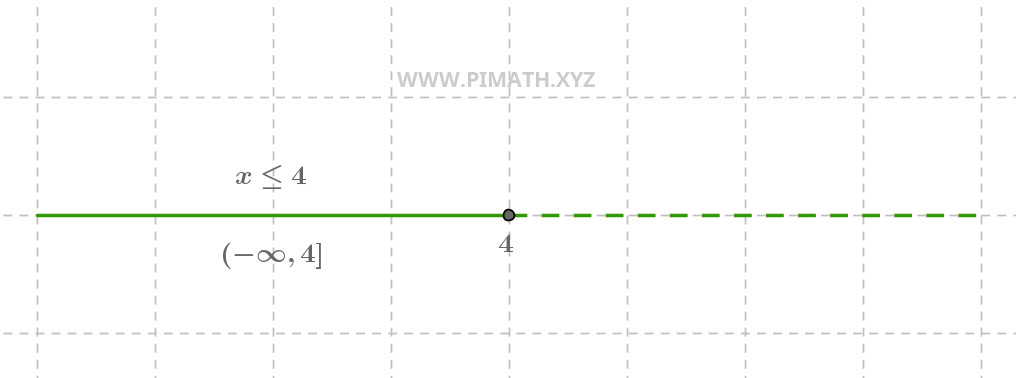
On the number line, we see a closed circle at \( 4 \) (because \( 4 \) is included) and a ray that starts from \( -\infty \) and goes to \( 4 \).

Example 2. Solution \( x > -2 \).

The solution \( x > -2 \) implies that all numbers greater than \( -2 \) are solutions. The graphical representation is as follows:

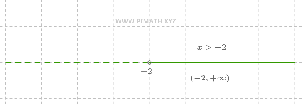
On the number line, we see an open circle at \( -2 \) (because \( -2 \) is not included) and a continuous line that starts from \( -2 \) and goes to \( +\infty \).

Example 3. Solution \( -2 \leq x < 5 \)

The solution \( -2 \leq x < 5 \) is an interval that includes \( -2 \) but excludes \( 5 \). The graphical representation is as follows:

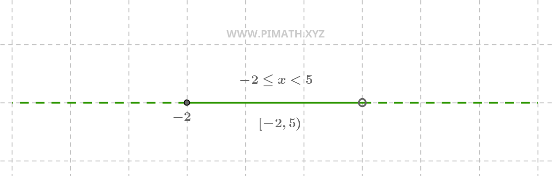
On the number line, we see a closed circle at \( -2 \) and an open circle at \( 5 \), with a continuous line between them.

The graphical interpretation of these solutions visually shows which values satisfy the inequality, making it easy for students to see the solution set.