Infinite Limits and Limits at Infinity: Definitions, Properties and Examples

Infinite limits and limits at infinity: a fundamental distinction

The expressions infinite limit and limit at infinity describe two distinct features of a limit. The first concerns the behaviour of the values of the function \(f(x)\); the second concerns instead the behaviour of the independent variable \(x\).

We speak of an infinite limit when

\[ f(x)\to+\infty \qquad\text{or}\qquad f(x)\to-\infty. \]

This is not to say that the function attains some value called \(+\infty\) or \(-\infty\). The symbols \(+\infty\) and \(-\infty\) are not real numbers: they indicate that the values of the function exceed any positive threshold, or fall below any negative threshold.

For example,

\[ \lim_{x\to2}\frac{1}{(x-2)^2}=+\infty \]

is an infinite limit, since the values of the function increase without bound as \(x\) approaches \(2\).

We speak instead of a limit at infinity when it is the variable \(x\) that tends to \(+\infty\) or to \(-\infty\). For example,

\[ \lim_{x\to+\infty}\frac{1}{x}=0 \]

is a limit at infinity, because \(x\) takes arbitrarily large positive values while the function tends to the finite value \(0\).

The two notions are independent

A limit can be infinite without being a limit at infinity. This is what happens, for instance, in

\[ \lim_{x\to0}\frac{1}{x^2}=+\infty. \]

Here \(x\) tends to the real number \(0\), while it is the function that tends to \(+\infty\).

Conversely, a limit can be at infinity without being infinite. For example,

\[ \lim_{x\to+\infty}\frac{2x+1}{x+1}=2. \]

Here \(x\to+\infty\), but the function tends to the real number \(2\).

Finally, the two features can occur together. The expression

\[ \lim_{x\to+\infty}x^2=+\infty \]

represents both a limit at infinity, since \(x\to+\infty\), and an infinite limit, since \(x^2\to+\infty\).

The four fundamental cases

Combining the behaviour of the variable with that of the function yields four fundamental cases.

1. Finite limit at a point: \(x\) tends to a real number \(x_0\) and \(f(x)\) tends to a real number \(L\): \[ \lim_{x\to x_0}f(x)=L. \]
2. Infinite limit at a point: \(x\) tends to a real number \(x_0\) and \(f(x)\) tends to \(+\infty\) or to \(-\infty\): \[ \lim_{x\to x_0}f(x)=\pm\infty. \]
3. Finite limit at infinity: \(x\) tends to \(+\infty\) or to \(-\infty\) and \(f(x)\) tends to a real number \(L\): \[ \lim_{x\to\pm\infty}f(x)=L. \]
4. Infinite limit at infinity: \(x\) tends to \(+\infty\) or to \(-\infty\) and \(f(x)\) likewise tends to \(+\infty\) or to \(-\infty\): \[ \lim_{x\to+\infty}f(x)=\pm\infty \qquad\text{or}\qquad \lim_{x\to-\infty}f(x)=\pm\infty. \]

It is therefore important to observe separately what happens to the variable and what happens to the values of the function. This distinction makes it possible to recognise at once the type of limit under study and to select the appropriate formal definition.

The meaning of the symbols \(+\infty\) and \(-\infty\)

In the theory of limits, the symbols \(+\infty\) and \(-\infty\) describe a behaviour, not a value attained by the function. Writing

\[ f(x)\to+\infty \]

means that \(f(x)\) eventually exceeds any prescribed positive real threshold. Similarly,

\[ f(x)\to-\infty \]

means that \(f(x)\) eventually falls below any prescribed negative real threshold.

The formal definitions given in the following sections will make these statements precise by means of suitable quantifiers and inequalities.

Infinite limits at a point

Let \(f:D\to\mathbb{R}\) and let \(x_0\) be an accumulation point of the domain \(D\). An infinite limit at \(x_0\) describes a situation in which the values of the function exceed any positive threshold, or fall below any negative threshold, as \(x\) approaches \(x_0\).

Two cases may arise:

\[ \lim_{x\to x_0}f(x)=+\infty \]

and

\[ \lim_{x\to x_0}f(x)=-\infty. \]

Limit equal to \(+\infty\)

Writing

\[ \lim_{x\to x_0}f(x)=+\infty \]

means that \(f(x)\) exceeds any prescribed positive threshold whenever \(x\) is sufficiently close to \(x_0\).

Formally,

\[ \forall M>0\ \exists\delta>0\ \forall x\in D: \quad 0<|x-x_0|<\delta \Longrightarrow f(x)>M. \]

The threshold \(M\) may be chosen arbitrarily large. Once \(M\) has been fixed, it must be possible to find a number \(\delta>0\) such that every point of the domain satisfying

\[ 0<|x-x_0|<\delta \]

has image greater than \(M\).

The number \(\delta\) may depend on \(M\): ever higher thresholds may require \(x\) to be chosen ever closer to \(x_0\).

Limit equal to \(-\infty\)

Similarly,

\[ \lim_{x\to x_0}f(x)=-\infty \]

means that \(f(x)\) falls below any prescribed negative threshold whenever \(x\) is sufficiently close to \(x_0\).

A particularly convenient formulation again makes use of a positive threshold \(M\):

\[ \forall M>0\ \exists\delta>0\ \forall x\in D: \quad 0<|x-x_0|<\delta \Longrightarrow f(x)<-M. \]

As \(M\) increases, the number \(-M\) becomes ever smaller. The definition thus requires the function eventually to fall below any prescribed negative level.

The value of the function at \(x_0\)

Whatever value the function may take at the point \(x_0\) plays no part in the definition of the limit. The condition

\[ 0<|x-x_0| \]

excludes, precisely, \(x=x_0\).

The function may therefore be undefined at \(x_0\), or it may be defined there and take any value whatsoever. The limit depends exclusively on the behaviour of \(f(x)\) at points of the domain arbitrarily close to \(x_0\).

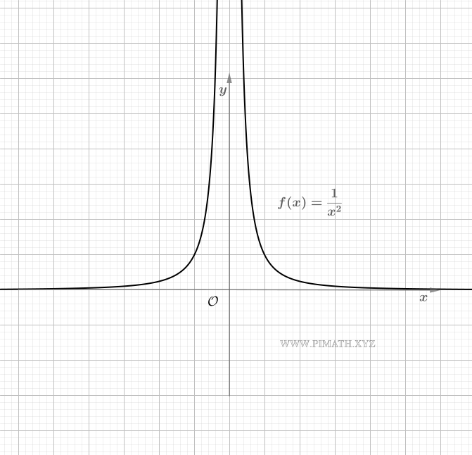
Example: \(\displaystyle\frac{1}{x^2}\) as \(x\to0\)

Consider

\[ f(x)=\frac{1}{x^2}, \qquad x\neq0. \]

As \(x\) approaches \(0\), the number \(x^2\) remains positive and tends to \(0\). Its reciprocal therefore becomes arbitrarily large:

\[ \lim_{x\to0}\frac{1}{x^2}=+\infty. \]

Let us verify this directly from the definition. Having fixed \(M>0\), we wish to obtain

\[ \frac{1}{x^2}>M. \]

Since \(x^2>0\) and \(M>0\), this inequality is equivalent to

\[ x^2<\frac{1}{M}, \]

that is,

\[ |x|<\frac{1}{\sqrt{M}}. \]

It therefore suffices to choose

\[ \delta=\frac{1}{\sqrt{M}}. \]

If

\[ 0<|x|<\delta, \]

then

\[ |x|<\frac{1}{\sqrt{M}}, \]

and hence

\[ \frac{1}{x^2}>M. \]

Since this construction is possible for every \(M>0\), the definition is verified.

Immagine

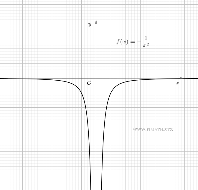
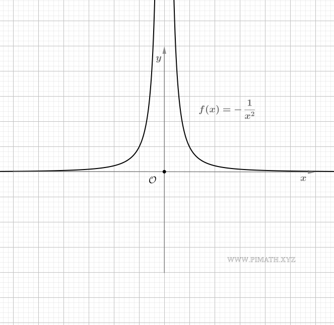
Example: \(-\displaystyle\frac{1}{x^2}\) as \(x\to0\)

Consider now

\[ f(x)=-\frac{1}{x^2}, \qquad x\neq0. \]

Since

\[ \frac{1}{x^2}\to+\infty, \]

changing sign, we obtain

\[ \lim_{x\to0}\left(-\frac{1}{x^2}\right)=-\infty. \]

This result, too, can be verified directly. Having fixed \(M>0\), we want

\[ -\frac{1}{x^2}<-M. \]

Multiplying by \(-1\) and reversing the direction of the inequality, we obtain

\[ \frac{1}{x^2}>M. \]

As in the previous example, it therefore suffices to choose

\[ \delta=\frac{1}{\sqrt{M}}. \]

It follows that, for every \(M>0\),

\[ 0<|x|<\delta \Longrightarrow -\frac{1}{x^2}<-M, \]

and hence

\[ \lim_{x\to0}\left(-\frac{1}{x^2}\right)=-\infty. \]

Immagine

A common error to avoid

For the limit to equal \(+\infty\) it is not enough for the function to take very large values only at certain points as they approach \(x_0\). Once a threshold \(M>0\) has been fixed, the inequality

\[ f(x)>M \]

must hold at every point of the domain sufficiently close to \(x_0\), with \(x_0\) itself excluded.

Similarly, for the limit to equal \(-\infty\), the function must eventually be less than \(-M\) for every threshold \(M>0\).

The symbols \(+\infty\) and \(-\infty\) thus describe a precise behaviour of the function, and not values actually attained.

An infinite limit does not imply monotonicity

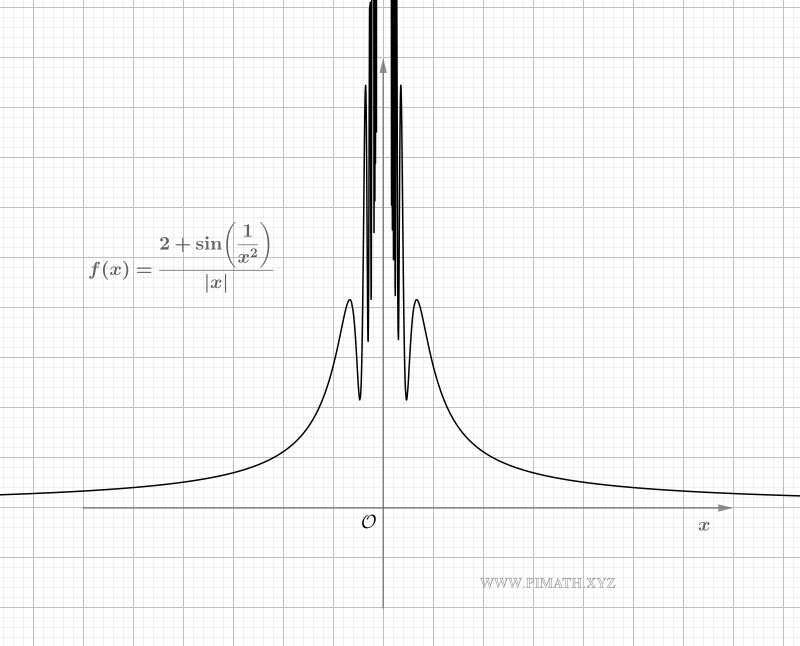
The existence of an infinite limit does not require the function to be monotonic near the point in question. A function may oscillate, even infinitely often, while still eventually exceeding every prescribed positive threshold.

Consider, for example,

\[ f(x)=\frac{2+\sin\left(\displaystyle\frac{1}{x^2}\right)}{|x|}, \qquad x\neq0. \]

Since

\[ 1\leq2+\sin\left(\frac{1}{x^2}\right)\leq3, \]

we have

\[ f(x)\geq\frac{1}{|x|}. \]

Moreover,

\[ \lim_{x\to0}\frac{1}{|x|}=+\infty. \]

By the comparison theorem it therefore follows that

\[ \lim_{x\to0}f(x)=+\infty. \]

The oscillating term prevents the function from being monotonic near \(0\), but does not prevent it from tending to \(+\infty\).

Immagine

Infinite right-hand and left-hand limits

When the behaviour of a function near a point \(x_0\) depends on the side from which \(x\) approaches, it is necessary to distinguish the right-hand limit from the left-hand limit.

In the right-hand limit, \(x\) approaches \(x_0\) through values greater than \(x_0\); in the left-hand limit, by contrast, through values less than \(x_0\).

One-sided limits, too, may be infinite. The four fundamental possibilities are

\[ \lim_{x\to x_0^+}f(x)=+\infty, \qquad \lim_{x\to x_0^+}f(x)=-\infty, \]

\[ \lim_{x\to x_0^-}f(x)=+\infty, \qquad \lim_{x\to x_0^-}f(x)=-\infty. \]

Infinite right-hand limit

Suppose that \(x_0\) is an accumulation point of the domain \(D\) from the right. We say that

\[ \lim_{x\to x_0^+}f(x)=+\infty \]

if, for every \(M>0\), there exists \(\delta>0\) such that, for every \(x\in D\),

\[ 0<x-x_0<\delta \quad\Longrightarrow\quad f(x)>M. \]

The condition

\[ 0<x-x_0<\delta \]

is equivalent to

\[ x_0<x<x_0+\delta, \]

so that only points of the domain lying to the right of \(x_0\) are taken into account.

Similarly,

\[ \lim_{x\to x_0^+}f(x)=-\infty \]

if, for every \(M>0\), there exists \(\delta>0\) such that

\[ 0<x-x_0<\delta \quad\Longrightarrow\quad f(x)<-M \]

for every \(x\in D\).

Infinite left-hand limit

Suppose now that \(x_0\) is an accumulation point of the domain \(D\) from the left. We say that

\[ \lim_{x\to x_0^-}f(x)=+\infty \]

if, for every \(M>0\), there exists \(\delta>0\) such that, for every \(x\in D\),

\[ 0<x_0-x<\delta \quad\Longrightarrow\quad f(x)>M. \]

In this case

\[ 0<x_0-x<\delta \]

is equivalent to

\[ x_0-\delta<x<x_0, \]

so that only points of the domain lying to the left of \(x_0\) are taken into account.

Similarly,

\[ \lim_{x\to x_0^-}f(x)=-\infty \]

if, for every \(M>0\), there exists \(\delta>0\) such that

\[ 0<x_0-x<\delta \quad\Longrightarrow\quad f(x)<-M. \]

Relation to the limit as \(x\to x_0\)

Suppose that \(x_0\) is an accumulation point of the domain both from the left and from the right. In this case,

\[ \lim_{x\to x_0}f(x)=+\infty \]

if and only if

\[ \lim_{x\to x_0^-}f(x)=+\infty \qquad\text{and}\qquad \lim_{x\to x_0^+}f(x)=+\infty. \]

Similarly,

\[ \lim_{x\to x_0}f(x)=-\infty \]

if and only if

\[ \lim_{x\to x_0^-}f(x)=-\infty \qquad\text{and}\qquad \lim_{x\to x_0^+}f(x)=-\infty. \]

If the two one-sided limits are infinite but of opposite sign, the limit as \(x\to x_0\) does not exist.

If, on the other hand, the domain contains points arbitrarily close to \(x_0\) only on one side, the limit must be interpreted relative to the domain, and coincides with the limit computed on the side on which such points occur.

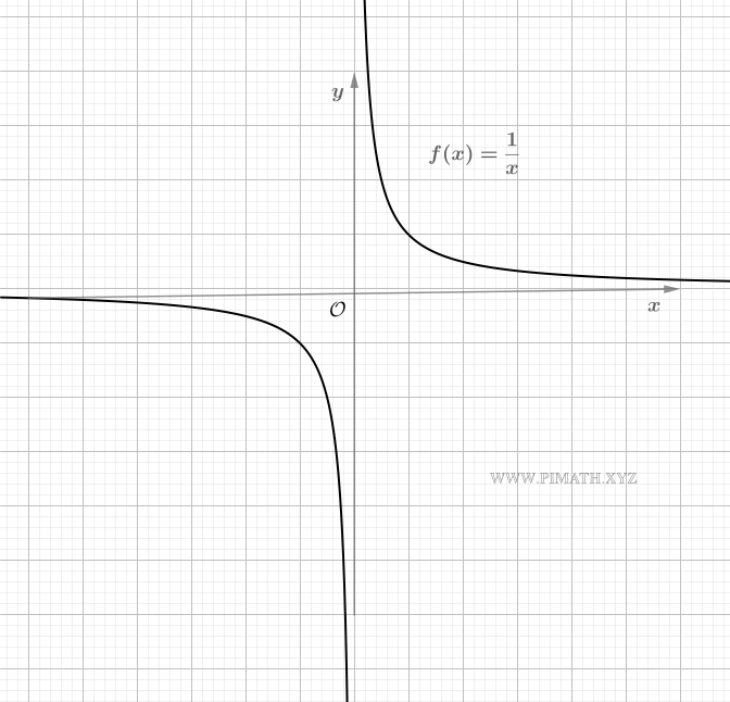
A fundamental example: the function \(\displaystyle\frac{1}{x}\)

Consider

\[ f(x)=\frac{1}{x}, \qquad x\neq0. \]

As \(x\) approaches \(0\) from the right, \(x\) is positive and tends to \(0\). Its reciprocal therefore becomes positive and arbitrarily large:

\[ \lim_{x\to0^+}\frac{1}{x}=+\infty. \]

As \(x\) approaches \(0\) from the left, on the other hand, \(x\) is negative and tends to \(0\). The reciprocal becomes negative and arbitrarily large in absolute value:

\[ \lim_{x\to0^-}\frac{1}{x}=-\infty. \]

The two one-sided limits therefore have opposite sign. Consequently,

\[ \lim_{x\to0}\frac{1}{x} \]

does not exist.

Immagine

Formal verification of the two one-sided limits

For the right-hand limit, fix \(M>0\). We want

\[ \frac{1}{x}>M. \]

Since \(x>0\), this inequality is equivalent to

\[ x<\frac{1}{M}. \]

It therefore suffices to choose

\[ \delta=\frac{1}{M}. \]

Indeed,

\[ 0<x<\delta \quad\Longrightarrow\quad x<\frac{1}{M} \quad\Longrightarrow\quad \frac{1}{x}>M. \]

For the left-hand limit, with the same choice

\[ \delta=\frac{1}{M}, \]

from the condition

\[ 0<-x<\delta \]

it follows that

\[ -\frac{1}{M}<x<0. \]

Since \(x\) is negative, taking reciprocals we obtain

\[ \frac{1}{x}<-M. \]

Both definitions are thus verified:

\[ \lim_{x\to0^+}\frac{1}{x}=+\infty, \qquad \lim_{x\to0^-}\frac{1}{x}=-\infty. \]

Geometric interpretation and vertical asymptotes

Infinite limits at a point admit an immediate geometric interpretation. As \(x\) approaches a real number \(x_0\) and \(f(x)\) tends to \(+\infty\) or to \(-\infty\), the points of the graph approach the vertical line

\[ x=x_0 \]

while their ordinates increase or decrease without bound.

In particular, if

\[ \lim_{x\to x_0}f(x)=+\infty, \]

then, for any fixed height \(M>0\), for \(x\) sufficiently close to \(x_0\) we have

\[ f(x)>M. \]

The graph thus lies above any horizontal line \(y=M\), provided \(x\) is sufficiently close to \(x_0\).

Similarly, if

\[ \lim_{x\to x_0}f(x)=-\infty, \]

then, for every \(M>0\), on approaching \(x_0\) sufficiently closely we have

\[ f(x)<-M. \]

In this case the graph descends below any horizontal line \(y=-M\).

Vertical asymptotes

This situation leads naturally to the concept of a vertical asymptote.

Let \(f:D\to\mathbb{R}\) and let \(x_0\in\mathbb{R}\) be an accumulation point of the domain from at least one of the two sides. The line

\[ x=x_0 \]

is called a vertical asymptote of the graph of \(f\) if at least one of the one-sided limits

\[ \lim_{x\to x_0^-}f(x), \qquad \lim_{x\to x_0^+}f(x) \]

equals \(+\infty\) or \(-\infty\).

It is therefore not necessary for the function to display the same behaviour on both sides. It suffices that, from at least one side, the values of the function increase or decrease without bound.

The limit may fail to exist

The existence of a vertical asymptote does not necessarily imply the existence of the limit as \(x\to x_0\).

For example, for

\[ f(x)=\frac{1}{x} \]

we have

\[ \lim_{x\to0^-}\frac{1}{x}=-\infty, \qquad \lim_{x\to0^+}\frac{1}{x}=+\infty. \]

The two one-sided limits have opposite sign, so

\[ \lim_{x\to0}\frac{1}{x} \]

does not exist. Nevertheless, the line

\[ x=0 \]

is a vertical asymptote of the graph.

The behaviour may occur on only one side

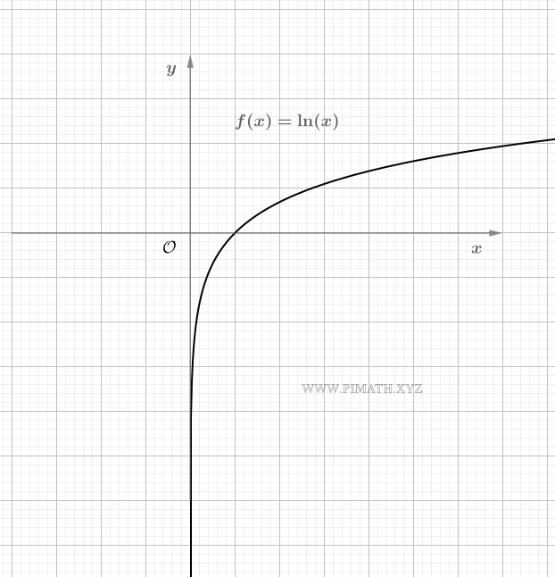
A vertical asymptote may also arise from a single one-sided limit. A fundamental example is the logarithmic function

\[ f(x)=\ln(x), \qquad x>0. \]

As \(x\to0^+\),

\[ \lim_{x\to0^+}\ln(x)=-\infty. \]

The function is not defined for \(x\leq0\), so there are no points of the domain arbitrarily close to \(0\) from the left. The infinite right-hand limit is nonetheless sufficient to conclude that

\[ x=0 \]

is a vertical asymptote.

Immagine

The point \(x_0\) may belong to the domain

The presence of a vertical asymptote does not require the function to be undefined at \(x_0\). Whatever value the function may take at that point does not, in fact, alter the behaviour of the limit.

Consider, for example,

\[ f(x)= \begin{cases} \displaystyle\frac{1}{x^2}, & x\neq0,\\ 0, & x=0. \end{cases} \]

The function is defined at \(x=0\), but

\[ \lim_{x\to0}f(x)=+\infty. \]

Consequently, the line \(x=0\) remains a vertical asymptote, regardless of the value assigned to \(f(0)\).

Immagine

The vanishing of the denominator is not sufficient

In rational functions, the vanishing of the denominator at a point does not automatically imply the presence of a vertical asymptote.

Consider

\[ f(x)=\frac{x^2-1}{x-1}. \]

The denominator vanishes at \(x=1\), but for \(x\neq1\) we may simplify:

\[ \frac{x^2-1}{x-1} = \frac{(x-1)(x+1)}{x-1} = x+1. \]

Hence,

\[ \lim_{x\to1}\frac{x^2-1}{x-1}=2. \]

The limit is finite, so \(x=1\) is not a vertical asymptote. The vanishing of the denominator must always be accompanied by an actual study of the limit.

An example with infinite behaviour on both sides

For the function

\[ f(x)=\frac{1}{(x-2)^2}, \]

the denominator tends to \(0\) through positive values both as \(x\to2^-\) and as \(x\to2^+\). We thus have

\[ \lim_{x\to2^-}\frac{1}{(x-2)^2}=+\infty, \qquad \lim_{x\to2^+}\frac{1}{(x-2)^2}=+\infty. \]

Consequently,

\[ \lim_{x\to2}\frac{1}{(x-2)^2}=+\infty, \]

and the line

\[ x=2 \]

is a vertical asymptote of the graph.

Immagine

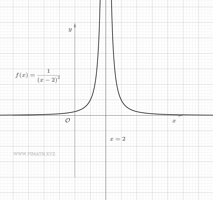
From a geometric standpoint, then, a vertical asymptote identifies a line which the graph approaches horizontally while the ordinates become arbitrarily large in absolute value on at least one of the two sides.

Finite limits as \(x\to+\infty\) and \(x\to-\infty\)

A finite limit at infinity describes the behaviour of a function as the variable \(x\) tends to \(+\infty\) or to \(-\infty\), while \(f(x)\) approaches a real number \(L\).

The two cases

\[ \lim_{x\to+\infty}f(x)=L \qquad\text{and}\qquad \lim_{x\to-\infty}f(x)=L \]

must be distinguished, because the behaviour of the function for very large positive values may differ from that observed for values that are very large in absolute value but negative.

Finite limit as \(x\to+\infty\)

In order to consider the limit as \(x\to+\infty\), the domain \(D\) of the function must be unbounded above, that is, it must contain arbitrarily large elements.

Let \(f:D\to\mathbb{R}\), with \(D\) unbounded above, and let \(L\in\mathbb{R}\). We say that

\[ \lim_{x\to+\infty}f(x)=L \]

if, for every \(\varepsilon>0\), there exists \(A\in\mathbb{R}\) such that, for every \(x\in D\),

\[ x>A \quad\Longrightarrow\quad |f(x)-L|<\varepsilon. \]

In symbolic form,

\[ \forall\varepsilon>0\ \exists A\in\mathbb{R}\ \forall x\in D: \quad x>A \Longrightarrow |f(x)-L|<\varepsilon. \]

The number \(\varepsilon\) establishes the precision with which \(f(x)\) must approximate \(L\), while \(A\) determines how large \(x\) must be for this precision to be guaranteed.

The condition

\[ |f(x)-L|<\varepsilon \]

is equivalent to

\[ L-\varepsilon<f(x)<L+\varepsilon. \]

Hence, for \(x\) sufficiently large, the values of the function remain arbitrarily close to \(L\).

Finite limit as \(x\to-\infty\)

To consider the limit as \(x\to-\infty\), the domain \(D\) must instead be unbounded below, that is, it must contain arbitrarily small elements.

Let \(f:D\to\mathbb{R}\), with \(D\) unbounded below, and let \(L\in\mathbb{R}\). We say that

\[ \lim_{x\to-\infty}f(x)=L \]

if, for every \(\varepsilon>0\), there exists \(A\in\mathbb{R}\) such that, for every \(x\in D\),

\[ x<A \quad\Longrightarrow\quad |f(x)-L|<\varepsilon. \]

In symbolic form,

\[ \forall\varepsilon>0\ \exists A\in\mathbb{R}\ \forall x\in D: \quad x<A \Longrightarrow |f(x)-L|<\varepsilon. \]

Here too, \(\varepsilon\) may be chosen arbitrarily small. The threshold \(A\) must be such that all points of the domain lying sufficiently far to the left produce values of \(f(x)\) within a distance \(\varepsilon\) of \(L\).

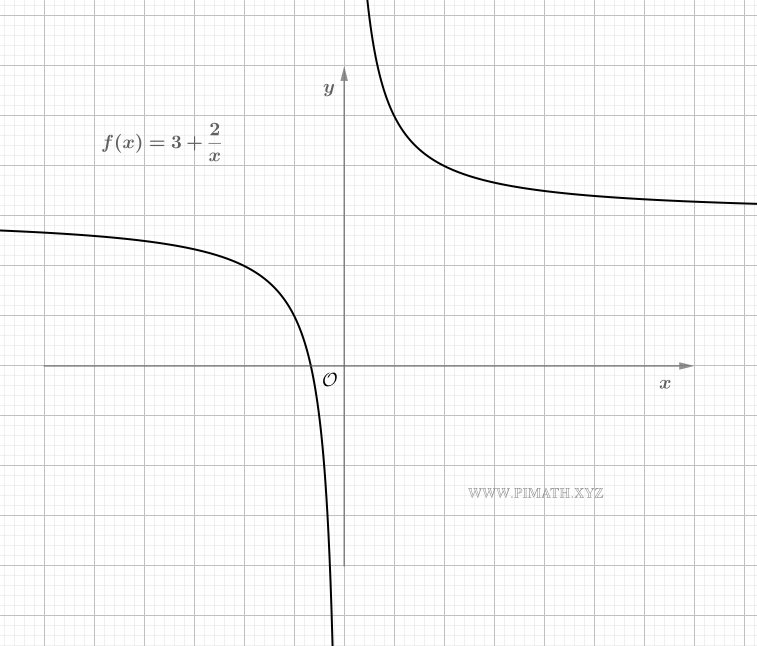
Example: the limit of \(3+\displaystyle\frac{2}{x}\)

Consider

\[ f(x)=3+\frac{2}{x}. \]

Since

\[ \lim_{x\to+\infty}\frac{2}{x}=0 \qquad\text{and}\qquad \lim_{x\to-\infty}\frac{2}{x}=0, \]

we have

\[ \lim_{x\to+\infty}\left(3+\frac{2}{x}\right)=3 \]

and

\[ \lim_{x\to-\infty}\left(3+\frac{2}{x}\right)=3. \]

We may verify the first limit directly. Having fixed \(\varepsilon>0\), we impose

\[ \left|3+\frac{2}{x}-3\right|<\varepsilon. \]

For \(x>0\), this condition is equivalent to

\[ \frac{2}{x}<\varepsilon, \]

and hence to

\[ x>\frac{2}{\varepsilon}. \]

It therefore suffices to choose

\[ A=\frac{2}{\varepsilon}. \]

As \(x\to-\infty\), on the other hand, from the condition

\[ \left|\frac{2}{x}\right|<\varepsilon \]

it suffices to require

\[ x<-\frac{2}{\varepsilon}. \]

The two formal definitions thus lead to the same value \(L=3\).

Immagine

The two limits may differ

The existence of a limit as \(x\to+\infty\) does not determine the behaviour of the function as \(x\to-\infty\). The two limits must be studied separately.

Consider, for example,

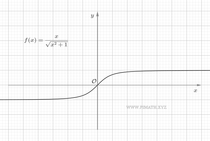
\[ f(x)=\frac{x}{\sqrt{x^2+1}}. \]

Since

\[ \sqrt{x^2+1} = |x|\sqrt{1+\frac{1}{x^2}}, \]

as \(x\to+\infty\) we eventually have \(|x|=x\), and hence

\[ \frac{x}{\sqrt{x^2+1}} = \frac{1}{\sqrt{1+\displaystyle\frac{1}{x^2}}} \to1. \]

As \(x\to-\infty\), on the other hand, we eventually have \(|x|=-x\), so

\[ \frac{x}{\sqrt{x^2+1}} = -\frac{1}{\sqrt{1+\displaystyle\frac{1}{x^2}}} \to-1. \]

Hence,

\[ \lim_{x\to+\infty}\frac{x}{\sqrt{x^2+1}}=1, \qquad \lim_{x\to-\infty}\frac{x}{\sqrt{x^2+1}}=-1. \]

Immagine

The limit does not describe the whole graph

A finite limit at infinity concerns exclusively the eventual behaviour of the function. Modifying \(f\) on a bounded set does not change its limit as \(x\to+\infty\) or as \(x\to-\infty\).

Moreover, the existence of a finite limit does not imply that the function is monotonic. For example,

\[ f(x)=\frac{\sin(x)}{x} \]

continues to oscillate, yet

\[ \left|\frac{\sin(x)}{x}\right| \leq \frac{1}{|x|}, \]

and since

\[ \lim_{x\to\pm\infty}\frac{1}{|x|}=0, \]

the comparison theorem gives

\[ \lim_{x\to\pm\infty}\frac{\sin(x)}{x}=0. \]

Immagine

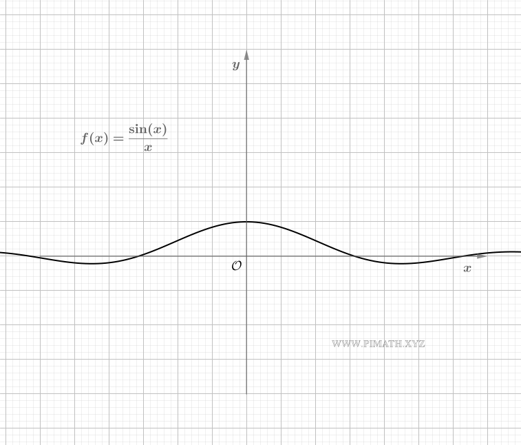
To say that \(x\to+\infty\) or \(x\to-\infty\) does not, therefore, mean that \(x\) attains some value called infinity. It means that the variable exceeds any prescribed positive threshold, or falls below any prescribed negative threshold, while the values of the function approach the real number \(L\) arbitrarily closely.

Geometric interpretation and horizontal asymptotes

When a function tends to a real number \(L\) as \(x\to+\infty\) or as \(x\to-\infty\), the points of its graph approach the horizontal line

\[ y=L. \]

Indeed, the condition

\[ |f(x)-L|<\varepsilon \]

means that the vertical distance between the point of the graph \((x,f(x))\) and the line \(y=L\) is less than \(\varepsilon\).

Since \(\varepsilon\) may be chosen arbitrarily small, this distance tends to zero in the direction under consideration.

Definition of a horizontal asymptote

Let \(f:D\to\mathbb{R}\). If

\[ \lim_{x\to+\infty}f(x)=L, \]

with \(L\in\mathbb{R}\), the line

\[ y=L \]

is called the right horizontal asymptote of the graph of \(f\).

If instead

\[ \lim_{x\to-\infty}f(x)=L, \]

then the same line

\[ y=L \]

is called the left horizontal asymptote.

When it is not necessary to specify the direction, one speaks simply of a horizontal asymptote.

Interpretation by means of horizontal strips

Suppose that

\[ \lim_{x\to+\infty}f(x)=L. \]

For every \(\varepsilon>0\), there exists a threshold \(A\) such that

\[ L-\varepsilon<f(x)<L+\varepsilon \]

for every \(x\in D\) with \(x>A\).

Geometrically, the graph thus lies eventually within the strip bounded by the lines

\[ y=L-\varepsilon \qquad\text{and}\qquad y=L+\varepsilon. \]

As \(x\to-\infty\) the same interpretation holds, with the difference that the condition is required for all \(x\in D\) that are sufficiently negative.

Approach from above, from below, or with oscillation

The graph need not always approach the asymptote from the same side.

For example,

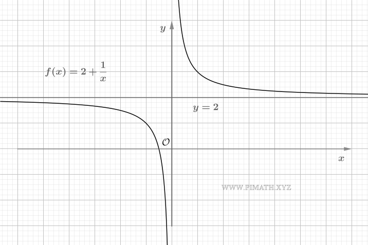
\[ f(x)=2+\frac{1}{x} \]

satisfies, for \(x>0\),

\[ f(x)>2 \]

and

\[ \lim_{x\to+\infty}\left(2+\frac{1}{x}\right)=2. \]

The graph therefore approaches the line \(y=2\) from above.

Similarly,

\[ f(x)=2-\frac{1}{x} \]

satisfies \(f(x)<2\) for \(x>0\) and likewise tends to \(2\). In this case the graph approaches the asymptote from below.

Immagine

An oscillating approach is also possible. For example,

\[ f(x)=L+\frac{\sin(x)}{x} \]

takes values alternately greater than and less than \(L\), yet

\[ \lim_{x\to+\infty}\left(L+\frac{\sin(x)}{x}\right)=L. \]

The existence of a horizontal asymptote does not, therefore, imply that the graph eventually remains on one fixed side of the line.

The same line may be an asymptote in both directions

If

\[ \lim_{x\to+\infty}f(x)=L \qquad\text{and}\qquad \lim_{x\to-\infty}f(x)=L, \]

the line \(y=L\) is a horizontal asymptote both on the right and on the left.

For example,

\[ f(x)=\frac{1}{x^2} \]

satisfies

\[ \lim_{x\to+\infty}\frac{1}{x^2}=0 \qquad\text{and}\qquad \lim_{x\to-\infty}\frac{1}{x^2}=0. \]

The line \(y=0\) is thus a horizontal asymptote in both directions.

A function may have two distinct horizontal asymptotes

The limits as \(x\to+\infty\) and as \(x\to-\infty\) may differ. If

\[ \lim_{x\to+\infty}f(x)=L_1 \qquad\text{and}\qquad \lim_{x\to-\infty}f(x)=L_2, \]

with \(L_1\neq L_2\), then \(y=L_1\) is the right horizontal asymptote and \(y=L_2\) is the left horizontal asymptote.

An example is

\[ f(x)=\frac{x}{\sqrt{x^2+1}}, \]

for which

\[ \lim_{x\to+\infty}\frac{x}{\sqrt{x^2+1}}=1, \qquad \lim_{x\to-\infty}\frac{x}{\sqrt{x^2+1}}=-1. \]

The lines \(y=1\) and \(y=-1\) are thus, respectively, the right and left horizontal asymptotes.

The graph may intersect the asymptote

A horizontal asymptote is not a line that the graph may never cross. The definition requires only that the vertical distance from the line tend to zero at infinity.

For example,

\[ f(x)=\frac{\sin(x)}{x} \]

has \(y=0\) as a horizontal asymptote, yet the graph crosses that line at

\[ x=k\pi, \qquad k\in\mathbb{Z}\setminus\{0\}. \]

In this case there are in fact infinitely many intersections.

Uniqueness of the asymptote in each direction

A function can have at most one horizontal asymptote as \(x\to+\infty\) and at most one as \(x\to-\infty\).

This follows from the uniqueness of the limit: if

\[ \lim_{x\to+\infty}f(x)=L_1 \qquad\text{and}\qquad \lim_{x\to+\infty}f(x)=L_2, \]

then necessarily \(L_1=L_2\). The same holds for \(x\to-\infty\).

How to find horizontal asymptotes

To determine the possible horizontal asymptotes of a function, one computes separately

\[ \lim_{x\to+\infty}f(x) \qquad\text{and}\qquad \lim_{x\to-\infty}f(x), \]

whenever the domain allows both limits to be considered.

If one of the two limits equals a real number \(L\), the line \(y=L\) is a horizontal asymptote in the corresponding direction. If, instead, the limit equals \(+\infty\), equals \(-\infty\), or fails to exist, there is no horizontal asymptote in that direction.

Infinite limits as \(x\to+\infty\) and \(x\to-\infty\)

An infinite limit at infinity occurs when the variable \(x\) tends to \(+\infty\) or to \(-\infty\) and, at the same time, the values of the function increase or decrease without bound.

Four cases may arise:

\[ \lim_{x\to+\infty}f(x)=+\infty, \qquad \lim_{x\to+\infty}f(x)=-\infty, \]

\[ \lim_{x\to-\infty}f(x)=+\infty, \qquad \lim_{x\to-\infty}f(x)=-\infty. \]

In each case it is necessary to distinguish the behaviour of the variable from that of the function: the sign of the infinity to which \(x\) tends does not determine the sign of the infinity to which \(f(x)\) tends.

Infinite limits as \(x\to+\infty\)

Let \(f:D\to\mathbb{R}\), with \(D\) unbounded above. We say that

\[ \lim_{x\to+\infty}f(x)=+\infty \]

if, for every \(M>0\), there exists \(A\in\mathbb{R}\) such that, for every \(x\in D\),

\[ x>A \quad\Longrightarrow\quad f(x)>M. \]

In symbolic form,

\[ \forall M>0\ \exists A\in\mathbb{R}\ \forall x\in D: \quad x>A \Longrightarrow f(x)>M. \]

The definition thus requires the function eventually to exceed any prescribed positive threshold.

Similarly,

\[ \lim_{x\to+\infty}f(x)=-\infty \]

if, for every \(M>0\), there exists \(A\in\mathbb{R}\) such that

\[ x>A \quad\Longrightarrow\quad f(x)<-M \]

for every \(x\in D\).

In this case, for sufficiently large values of \(x\), the function falls below any prescribed negative threshold.

Infinite limits as \(x\to-\infty\)

Suppose now that the domain \(D\) is unbounded below. We say that

\[ \lim_{x\to-\infty}f(x)=+\infty \]

if, for every \(M>0\), there exists \(A\in\mathbb{R}\) such that, for every \(x\in D\),

\[ x<A \quad\Longrightarrow\quad f(x)>M. \]

In symbolic form,

\[ \forall M>0\ \exists A\in\mathbb{R}\ \forall x\in D: \quad x<A \Longrightarrow f(x)>M. \]

Similarly,

\[ \lim_{x\to-\infty}f(x)=-\infty \]

if, for every \(M>0\), there exists \(A\in\mathbb{R}\) such that

\[ x<A \quad\Longrightarrow\quad f(x)<-M. \]

In this case the function falls below every prescribed negative threshold for all \(x\) in the domain that are sufficiently negative.

Fundamental examples involving powers

The function

\[ f(x)=x^2 \]

tends to \(+\infty\) in both directions:

\[ \lim_{x\to+\infty}x^2=+\infty, \qquad \lim_{x\to-\infty}x^2=+\infty. \]

Indeed, \(x^2\) becomes arbitrarily large as the absolute value of \(x\) increases, regardless of the sign of \(x\).

The cubic function

\[ f(x)=x^3 \]

displays, by contrast, different behaviour:

\[ \lim_{x\to+\infty}x^3=+\infty, \qquad \lim_{x\to-\infty}x^3=-\infty. \]

The sign of the term is, indeed, always that of \(x\).

The role of the parity of the exponent

More generally, the behaviour of the power \(x^n\), with \(n\) a positive integer, depends on the parity of the exponent.

As \(x\to+\infty\), we always have

\[ \lim_{x\to+\infty}x^n=+\infty. \]

As \(x\to-\infty\), on the other hand, if \(n\) is even,

\[ \lim_{x\to-\infty}x^n=+\infty, \]

whereas, if \(n\) is odd,

\[ \lim_{x\to-\infty}x^n=-\infty. \]

The coefficient multiplying the power can, naturally, alter the sign of the limit. For example,

\[ \lim_{x\to+\infty}(-x^2)=-\infty, \qquad \lim_{x\to-\infty}(-x^3)=+\infty. \]

Formal verification that \(\displaystyle\lim_{x\to+\infty}x^2=+\infty\)

Having fixed \(M>0\), we must find a threshold \(A\) such that

\[ x>A \quad\Longrightarrow\quad x^2>M. \]

For \(x>0\), the condition

\[ x^2>M \]

holds when

\[ x>\sqrt{M}. \]

We may therefore choose

\[ A=\sqrt{M}. \]

Since this choice is possible for every \(M>0\), it follows from the definition that

\[ \lim_{x\to+\infty}x^2=+\infty. \]

Formal verification that \(\displaystyle\lim_{x\to-\infty}x^3=-\infty\)

Having fixed \(M>0\), we wish to find \(A\in\mathbb{R}\) such that

\[ x<A \quad\Longrightarrow\quad x^3<-M. \]

Since the cubic function is strictly increasing,

\[ x^3<-M \]

is equivalent to

\[ x<-\sqrt[3]{M}. \]

It therefore suffices to choose

\[ A=-\sqrt[3]{M}. \]

It follows that

\[ \lim_{x\to-\infty}x^3=-\infty. \]

Geometric interpretation

If

\[ \lim_{x\to+\infty}f(x)=+\infty, \]

then, for any fixed horizontal line \(y=M\), with \(M>0\), the graph eventually lies above that line as we proceed to the right.

If instead

\[ \lim_{x\to+\infty}f(x)=-\infty, \]

the graph eventually lies below any line \(y=-M\).

The same interpretations hold as \(x\to-\infty\), proceeding instead to the left along the \(x\)-axis.

Unlike finite limits at infinity, in these cases there is no horizontal asymptote: the ordinates do not approach a real number, but increase or decrease without bound.

Fundamental properties of infinite limits and limits at infinity

The properties of limits often make it possible to determine the behaviour of sums, products and quotients without appealing directly to the formal definitions.

In what follows, the limits of \(f\) and \(g\) are always understood with respect to the same limiting process, which may be a limit at a point, a one-sided limit, or a limit at infinity.

Whenever \(+\infty\) and \(-\infty\) appear, however, it is essential to bear in mind that these symbols do not represent real numbers. Expressions such as

\[ +\infty+L=+\infty \]

must be interpreted as shorthand for properties concerning limits, not as ordinary arithmetic operations.

Persistence of sign

If a function tends to \(+\infty\), then it is eventually positive. Indeed, from the definition we may choose, for instance, \(M=1\); it follows that

\[ f(x)>1>0 \]

for all values of \(x\) sufficiently close to the point in question or, in limits at infinity, sufficiently large if \(x\to+\infty\) or sufficiently negative if \(x\to-\infty\).

Similarly, if

\[ f(x)\to-\infty, \]

then \(f(x)\) is eventually negative.

This property is particularly important in products and quotients, since it allows the sign of the result to be established correctly.

Sum with a finite limit

Suppose that, in the same limiting process,

\[ f(x)\to+\infty \qquad\text{and}\qquad g(x)\to L, \]

with \(L\in\mathbb{R}\). Then

\[ f(x)+g(x)\to+\infty. \]

Similarly,

\[ f(x)\to-\infty, \qquad g(x)\to L \]

implies

\[ f(x)+g(x)\to-\infty. \]

In symbolic form,

\[ +\infty+L=+\infty, \qquad -\infty+L=-\infty. \]

A term tending to a finite value therefore does not alter the infinite behaviour of the sum.

Sum of infinite limits

If two functions both tend to \(+\infty\), their sum tends to \(+\infty\):

\[ (+\infty)+(+\infty)=+\infty. \]

Similarly,

\[ (-\infty)+(-\infty)=-\infty. \]

The case in which the two terms have opposite sign is, however, different. The form

\[ \infty-\infty \]

is indeterminate: knowledge of the limits of the two terms alone does not allow the limit of the difference to be determined.

For example, as \(x\to+\infty\),

\[ x^2-x\to+\infty, \qquad x-x^2\to-\infty, \]

while

\[ (x+1)-x\to1. \]

In all these cases the two quantities being subtracted tend to \(+\infty\), yet the results differ.

Products

If one function tends to infinity and the other tends to a non-zero real number, the absolute value of the product tends to infinity, and its sign is determined by the usual rule of signs.

For example, if

\[ f(x)\to+\infty \qquad\text{and}\qquad g(x)\to L>0, \]

then

\[ f(x)g(x)\to+\infty. \]

If instead \(L<0\),

\[ f(x)g(x)\to-\infty. \]

When both factors tend to infinity, we likewise have

\[ (+\infty)(+\infty)=+\infty, \qquad (+\infty)(-\infty)=-\infty, \]

\[ (-\infty)(+\infty)=-\infty, \qquad (-\infty)(-\infty)=+\infty. \]

The situation changes if one of the factors tends to \(0\). The form

\[ 0\cdot\infty \]

is indeterminate and requires further study of the expression.

Quotient with infinite denominator

If

\[ f(x)\to L\in\mathbb{R} \]

and

\[ g(x)\to+\infty \qquad\text{or}\qquad g(x)\to-\infty, \]

then

\[ \frac{f(x)}{g(x)}\to0, \]

provided the quotient is eventually defined.

In particular, for a real constant \(L\),

\[ \frac{L}{\pm\infty}=0 \]

is a symbolic notation summarising this property.

If, instead, numerator and denominator both tend to infinity, the indeterminate form

\[ \frac{\infty}{\infty}. \]

arises. The result depends on the relative behaviour of numerator and denominator and cannot be established from the symbolic form alone.

Reciprocal

If

\[ f(x)\to+\infty \qquad\text{or}\qquad f(x)\to-\infty, \]

then

\[ \frac{1}{f(x)}\to0. \]

Conversely, if a function tends to zero while eventually keeping a fixed sign, its reciprocal tends to infinity with the corresponding sign:

\[ f(x)\to0^+ \quad\Longrightarrow\quad \frac{1}{f(x)}\to+\infty, \]

while

\[ f(x)\to0^- \quad\Longrightarrow\quad \frac{1}{f(x)}\to-\infty. \]

Checking the sign of the denominator is therefore essential whenever a quantity tends to zero.

The principal indeterminate forms

The indeterminate forms that occur most frequently in the study of limits are

\[ \frac{0}{0}, \qquad \frac{\infty}{\infty}, \qquad \infty-\infty, \qquad 0\cdot\infty. \]

An indeterminate form does not represent the value of the limit. It indicates merely that the elementary rules do not allow one to draw an immediate conclusion, and that the expression must be transformed or examined more closely.

For example,

\[ \frac{x}{x}\to1, \qquad \frac{x}{x^2}\to0, \qquad \frac{x^2}{x}\to+\infty \]

as \(x\to+\infty\), even though all three expressions initially present the form

\[ \frac{\infty}{\infty}. \]

To resolve such cases it is necessary to analyse the relative behaviour of the terms involved. In the next section we shall see how comparing functions and identifying the dominant term make it possible to deal with many such limits.

Comparison of functions and dominant behaviour

In limits at infinity it is often useful to identify which term determines the overall behaviour of an expression. This principle is especially important when indeterminate forms such as

\[ \frac{\infty}{\infty} \qquad\text{or}\qquad \infty-\infty \]

arise. The basic idea is to compare the terms present and identify the dominant one, that is, the term which carries decisive weight in the limit under consideration.

The dominant term of a polynomial

Consider a polynomial of degree \(n\):

\[ P(x)=a_nx^n+a_{n-1}x^{n-1}+\cdots+a_1x+a_0, \qquad a_n\neq0. \]

As \(x\to\pm\infty\), the behaviour of the polynomial is determined by the term of highest degree, \(a_nx^n\). Indeed, factoring out \(x^n\),

\[ P(x) = x^n \left( a_n+\frac{a_{n-1}}{x} +\frac{a_{n-2}}{x^2} +\cdots+ \frac{a_0}{x^n} \right). \]

All the terms containing powers of \(x\) in the denominator tend to \(0\). Consequently, the sign and the infinite behaviour of \(P(x)\) depend on the leading coefficient \(a_n\), on the parity of \(n\), and on the direction of the limit.

For example,

\[ P(x)=-2x^5+3x^2-1 \]

has \(-2x^5\) as its dominant term. Hence,

\[ \lim_{x\to+\infty}P(x)=-\infty, \qquad \lim_{x\to-\infty}P(x)=+\infty. \]

Rational functions

Consider a rational function

\[ f(x)=\frac{P(x)}{Q(x)}, \]

where \(P\) and \(Q\) are polynomials, with \(Q\) not identically zero. To study its behaviour at infinity it suffices to compare the terms of highest degree in the numerator and in the denominator.

If the degree of \(P\) is less than the degree of \(Q\), then

\[ \lim_{x\to\pm\infty}\frac{P(x)}{Q(x)}=0. \]

If the two polynomials have the same degree, the limit equals the ratio of their respective leading coefficients.

For example,

\[ \lim_{x\to\pm\infty} \frac{3x^2-x+1}{2x^2+5} = \frac{3}{2}. \]

If, instead, the degree of the numerator exceeds that of the denominator, the absolute value of the ratio grows without bound; the sign must be determined by studying the dominant terms.

For example,

\[ \frac{2x^3+1}{x^2-4} \]

behaves, for large values of \(|x|\), like \(2x\). Hence,

\[ \lim_{x\to+\infty}\frac{2x^3+1}{x^2-4}=+\infty, \qquad \lim_{x\to-\infty}\frac{2x^3+1}{x^2-4}=-\infty. \]

The comparison theorem

The behaviour of a function can also be deduced by comparing it with a simpler function.

If, eventually,

\[ f(x)\geq g(x) \]

and

\[ g(x)\to+\infty, \]

then

\[ f(x)\to+\infty. \]

Similarly, if eventually

\[ f(x)\leq g(x) \]

and

\[ g(x)\to-\infty, \]

then

\[ f(x)\to-\infty. \]

Comparison and the identification of the dominant term thus make it possible to resolve many limits at infinity without mechanically applying symbolic rules to indeterminate forms.

Examples of infinite limits and limits at infinity

We conclude with a number of representative examples that bring together the principal cases studied. The aim is to recognise the type of limit, identify the determining behaviour of the expression, and interpret the result geometrically whenever this is possible.

Example 1: an infinite limit at a point

Consider

\[ \lim_{x\to2}\frac{1}{(x-2)^2}. \]

As \(x\to2\), we have

\[ (x-2)^2\to0^+. \]

The denominator therefore tends to zero while remaining positive. Its reciprocal takes arbitrarily large positive values, and hence

\[ \lim_{x\to2}\frac{1}{(x-2)^2}=+\infty. \]

The same behaviour occurs on both sides:

\[ \lim_{x\to2^-}\frac{1}{(x-2)^2}=+\infty, \qquad \lim_{x\to2^+}\frac{1}{(x-2)^2}=+\infty. \]

The line

\[ x=2 \]

is thus a vertical asymptote.

Example 2: infinite one-sided limits of opposite sign

Consider

\[ \lim_{x\to1}\frac{1}{x-1}. \]

As \(x\to1^+\), the denominator tends to zero through positive values:

\[ x-1\to0^+. \]

Consequently,

\[ \lim_{x\to1^+}\frac{1}{x-1}=+\infty. \]

As \(x\to1^-\), on the other hand,

\[ x-1\to0^-, \]

and hence

\[ \lim_{x\to1^-}\frac{1}{x-1}=-\infty. \]

Since the two one-sided limits do not coincide,

\[ \lim_{x\to1}\frac{1}{x-1} \]

does not exist. The line \(x=1\) is nonetheless a vertical asymptote, since both one-sided limits are infinite.

Example 3: a finite limit at infinity and a horizontal asymptote

Let us compute

\[ \lim_{x\to+\infty}\frac{3x+1}{x+2}. \]

Both the numerator and the denominator tend to \(+\infty\), so the expression initially presents the indeterminate form

\[ \frac{\infty}{\infty}. \]

Dividing numerator and denominator by \(x\),

\[ \frac{3x+1}{x+2} = \frac{3+\displaystyle\frac{1}{x}} {1+\displaystyle\frac{2}{x}}. \]

Since

\[ \frac{1}{x}\to0 \qquad\text{as}\qquad x\to+\infty, \]

we obtain

\[ \lim_{x\to+\infty}\frac{3x+1}{x+2}=3. \]

The limit is finite, so the line

\[ y=3 \]

is a right horizontal asymptote.

Example 4: an infinite limit of a polynomial

Consider

\[ \lim_{x\to-\infty}\left(2x^4-3x^2+x-1\right). \]

The dominant term of the polynomial is

\[ 2x^4. \]

Since the exponent \(4\) is even,

\[ x^4\to+\infty \qquad\text{as}\qquad x\to-\infty. \]

Moreover, the leading coefficient is positive. The lower-degree terms do not affect the dominant behaviour, and hence

\[ \lim_{x\to-\infty}\left(2x^4-3x^2+x-1\right)=+\infty. \]

This example shows how, for polynomials, it generally suffices to identify the term of highest degree in order to determine the behaviour at infinity.

Example 5: the indeterminate form \(\infty-\infty\)

Let us compute

\[ \lim_{x\to+\infty}\left(\sqrt{x^2+x}-x\right). \]

We have

\[ \sqrt{x^2+x}\to+\infty \qquad\text{and}\qquad x\to+\infty, \]

so the indeterminate form

\[ \infty-\infty \]

arises. To remove it, we rationalise:

\[ \sqrt{x^2+x}-x = \frac{\left(\sqrt{x^2+x}-x\right) \left(\sqrt{x^2+x}+x\right)} {\sqrt{x^2+x}+x}. \]

In the numerator we obtain

\[ x^2+x-x^2=x, \]

and hence

\[ \sqrt{x^2+x}-x = \frac{x}{\sqrt{x^2+x}+x}. \]

Since, as \(x\to+\infty\), we eventually have \(x>0\), we may divide numerator and denominator by \(x\):

\[ \frac{x}{\sqrt{x^2+x}+x} = \frac{1} {\sqrt{1+\displaystyle\frac{1}{x}}+1}. \]

Passing to the limit,

\[ \lim_{x\to+\infty} \left(\sqrt{x^2+x}-x\right) = \frac{1}{2}. \]

The form \(\infty-\infty\) did not, therefore, represent the value of the limit: after a suitable algebraic transformation, a finite value is obtained.

Example 6: an infinite limit with an oscillating term

Consider

\[ f(x)=x+2\sin(x). \]

The term \(2\sin(x)\) oscillates continually, but remains bounded. Indeed,

\[ -1\leq\sin(x)\leq1, \]

and hence

\[ -2\leq2\sin(x)\leq2. \]

Adding \(x\),

\[ x-2\leq x+2\sin(x)\leq x+2. \]

In particular,

\[ x+2\sin(x)\geq x-2. \]

Since

\[ \lim_{x\to+\infty}(x-2)=+\infty, \]

the comparison theorem gives

\[ \lim_{x\to+\infty}\left(x+2\sin(x)\right)=+\infty. \]

This example is important because it shows that a function need not be monotonic in order to tend to \(+\infty\). Oscillation is compatible with an infinite limit, provided the function eventually exceeds any prescribed positive threshold.

Concluding scheme

In studying an infinite limit or a limit at infinity, it is useful to proceed in an orderly fashion:

1. identify the point, or the infinity, to which the variable tends;
2. if \(x\) tends to a real point, check whether it is necessary to distinguish the behaviour from the right and from the left;
3. carefully check the sign of any quantities tending to zero;
4. identify any indeterminate forms that arise;
5. identify, where possible, the dominant term, or apply a suitable comparison;
6. interpret the result geometrically, checking for the possible presence of vertical or horizontal asymptotes.

The formal definitions remain the foundation of the theory. The properties of limits, algebraic manipulations and comparisons allow one to recognise more quickly which of the behaviours described by the definitions occurs in the case at hand.