

Monomials and polynomials are among the foundational structures of elementary algebra. They are used to describe numerical relationships, geometric formulas, equations, and models that arise in virtually every branch of mathematics. Understanding their structure with precision is not merely a matter of learning computational techniques: it means grasping how algebraic expressions are built and what rules govern their transformations.
From a mathematical standpoint, polynomials are finite combinations of non-negative integer powers of variables, while monomials are the building blocks from which these combinations are assembled. Operations on monomials and polynomials follow directly from the properties of exponents and the distributivity of multiplication over addition.
A rigorous treatment requires careful attention to definitions: not every algebraic expression is a monomial or a polynomial, and many operational rules hold only under specific conditions on the exponents and variables involved.
Contents
- Definition of a Monomial
- Coefficient, Variable Part, and Degree
- Like Terms
- Operations on Monomials
- Definition of a Polynomial
- Degree of a Polynomial
- Operations on Polynomials
- Special Products and Algebraic Structure
- Evaluating a Polynomial
- Zeros of a Polynomial
- Ruffini's Rule
- Graphical Interpretation
Definition of a Monomial
A monomial is an expression of the form:
\[ a x_1^{\alpha_1}x_2^{\alpha_2}\cdots x_n^{\alpha_n}, \]
where:
- \( a \in \mathbb{R} \) is a real number called the coefficient;
- \( x_1, x_2, \dots, x_n \) are variables;
- \( \alpha_1, \alpha_2, \dots, \alpha_n \in \mathbb{N} \) are non-negative integer exponents.
The requirement that the exponents belong to \( \mathbb{N} \) is essential. Expressions such as:
\[ x^{-1}, \qquad \sqrt{x}, \qquad x^{1/2} \]
are not monomials, as they involve negative or fractional exponents.
A real number with no variables is also a monomial: for instance,
\[ 7 = 7x^0. \]
A monomial with a zero coefficient is called the zero monomial. Since:
\[ 0 \cdot x_1^{\alpha_1}\cdots x_n^{\alpha_n}=0, \]
all monomials with a zero coefficient represent the same zero expression.
Coefficient, Variable Part, and Degree
In the monomial:
\[ -5x^2y^3, \]
the number \( -5 \) is the coefficient, while:
\[ x^2y^3 \]
is the variable part.
The degree with respect to a variable is the exponent with which that variable appears. In the example above:
- the degree with respect to \( x \) is \( 2 \);
- the degree with respect to \( y \) is \( 3 \).
The total degree of a nonzero monomial is the sum of all its exponents:
\[ 2+3=5. \]
Thus:
\[ -5x^2y^3 \]
is a monomial of degree \( 5 \).
The degree of the zero monomial is generally left undefined, since the zero monomial can formally be written with any set of exponents.
Like Terms
Two monomials are called like terms if they share the same variable part — that is, if their variables appear with identical exponents.
For example:
\[ 3x^2y \qquad \text{and} \qquad -7x^2y \]
are like terms, whereas:
\[ 3x^2y \qquad \text{and} \qquad 3xy^2 \]
are not.
This notion is fundamental because only like terms can be combined algebraically.:
\[ 3x^2y-7x^2y=(3-7)x^2y=-4x^2y. \]
When two monomials are not like terms, their sum cannot be simplified further:
\[ x^2+x \]
is not a monomial.
Operations on Monomials
Operations on monomials follow directly from the properties of exponents.
Let:
\[ ax^\alpha y^\beta \qquad \text{and} \qquad bx^\gamma y^\delta. \]
Their product is:
\[ (ax^\alpha y^\beta)(bx^\gamma y^\delta) = ab\,x^{\alpha+\gamma}y^{\beta+\delta}. \]
This rule follows from the identity:
\[ x^\alpha x^\gamma=x^{\alpha+\gamma}. \]
For example:
\[ (2x^2y)(-3xy^4) = -6x^3y^5. \]
For the quotient:
\[ \frac{ax^\alpha}{bx^\beta} = \frac{a}{b}x^{\alpha-\beta}, \qquad b\neq0. \]
However, for the result to remain a monomial, it is required that:
\[ \alpha-\beta \ge 0. \]
Indeed:
\[ \frac{x^2}{x^5}=x^{-3} \]
is not a monomial.
Definition of a Polynomial
A polynomial is a finite sum of monomials.
In one variable, a polynomial takes the form:
\[ P(x)=a_0+a_1x+a_2x^2+\cdots+a_nx^n, \]
where:
- \( a_0,a_1,\dots,a_n \in \mathbb{R} \);
- \( n \in \mathbb{N} \);
- \( a_n\neq0 \).
The coefficient \( a_n \) is called the leading coefficient, while \( a_0 \) is the constant term.
For example:
\[ P(x)=2x^3-5x+1 \]
is a polynomial of degree three.
The following are not polynomials:
\[ \frac{1}{x}, \qquad \sqrt{x}, \qquad x^\pi, \qquad 2^x, \]
since they involve negative, fractional, or irrational exponents, or variables occurring in the exponent.
Degree of a Polynomial
The degree of a nonzero polynomial is the highest degree among its terms, after all like terms have been combined.
For example:
\[ P(x)=4x^5-2x^3+x-7 \]
has degree \( 5 \).
The polynomial:
\[ x^3-2x^3+x \]
simplifies to:
\[ -x^3+x, \]
and therefore still has degree \( 3 \).
The zero polynomial is the polynomial whose coefficients are all zero:
\[ 0. \]
Its degree is generally left undefined; in some advanced treatments it is conventionally set to:
\[ \deg(0)=-\infty. \]
Operations on Polynomials
The sum of two polynomials is obtained by combining like terms.
For example:
\[ (2x^2+3x-1)+(x^2-5x+4) \]
becomes:
\[ 3x^2-2x+3. \]
Multiplication relies on the distributive property:
\[ a(b+c)=ab+ac. \]
For example:
\[ (x+2)(x+5) \]
expands as:
\[ x(x+5)+2(x+5), \]
that is:
\[ x^2+5x+2x+10=x^2+7x+10. \]
The product of two polynomials is again a polynomial, since sums and products of monomials with non-negative integer exponents always yield monomials of the same kind.
Special Products and Algebraic Structure
Certain polynomial products arise so frequently that they are given standard forms, known as special products.
For example:
\[ (a+b)^2=a^2+2ab+b^2, \]
\[ (a-b)^2=a^2-2ab+b^2, \]
\[ (a+b)(a-b)=a^2-b^2. \]
These identities are not arbitrary formulas: they follow directly from the distributive property of multiplication over addition.
For example:
\[ (a+b)^2=(a+b)(a+b) \]
yields:
\[ a^2+ab+ab+b^2=a^2+2ab+b^2. \]
Evaluating a Polynomial
Every polynomial naturally defines a function.
For example:
\[ P(x)=x^2-3x+2 \]
assigns to every real number \( x \) the value:
\[ x^2-3x+2. \]
Evaluating a polynomial means substituting a real number for the variable.
For instance:
\[ P(4)=4^2-3\cdot4+2=16-12+2=6. \]
Since polynomials involve only sums and products, they are defined for every real number.
Zeros of a Polynomial
A zero of a polynomial \( P(x) \) is a real number \( x_0 \) such that:
\[ P(x_0)=0. \]
Finding the zeros of a polynomial is equivalent to solving a polynomial equation.
For example:
\[ x^2-5x+6=0 \]
factors as:
\[ (x-2)(x-3)=0, \]
and therefore has the zeros:
\[ x=2 \qquad \text{and} \qquad x=3. \]
For a monic polynomial — one with integer coefficients and leading coefficient \( 1 \) — any integer zeros must be divisors of the constant term \( a_0 \). This criterion reduces the search to a finite set of candidates, each of which can be tested by direct substitution.
Geometrically, the zeros of a polynomial correspond to the points where its graph crosses the \( x \)-axis.
Ruffini's Rule
Ruffini's rule (also known as synthetic division) is an algorithm for dividing a polynomial \( P(x) \) by a binomial of the form \( (x - r) \) in a fast and systematic way, using only the coefficients of \( P(x) \).
The theoretical foundation is the Remainder Theorem: dividing \( P(x) \) by \( (x-r) \) yields
\[ P(x) = (x-r)\,Q(x) + R, \]
where \( Q(x) \) is the quotient and \( R \) is a constant remainder. Substituting \( x = r \) gives immediately:
\[ P(r) = R. \]
This leads to the Factor Theorem: \( (x-r) \) divides \( P(x) \) with no remainder if and only if \( r \) is a zero of \( P(x) \), that is, \( P(r) = 0 \).
Procedure. Given the polynomial
\[ P(x) = a_n x^n + a_{n-1}x^{n-1} + \cdots + a_1 x + a_0, \]
the coefficients are arranged in a row and the computation proceeds as follows:
\[ \begin{array}{c|cccc} r & a_n & a_{n-1} & \cdots & a_0 \\ & & r\,b_n & \cdots & r\,b_1 \\ \hline & b_n & b_{n-1} & \cdots & R \end{array} \]
where \( b_n = a_n \) and, for \( k = n-1, \dots, 0 \):
\[ b_k = a_k + r\,b_{k+1}. \]
The values \( b_n, b_{n-1}, \dots, b_1 \) are the coefficients of the quotient polynomial \( Q(x) \) of degree \( n-1 \); the final value \( R \) is the remainder, which equals \( P(r) \).
Example. We wish to divide
\[ P(x) = x^3 - 6x^2 + 11x - 6 \]
by \( (x-1) \), thereby checking whether \( r = 1 \) is a zero.
\[ \begin{array}{c|cccc} 1 & 1 & -6 & 11 & -6 \\ & & 1 & -5 & 6 \\ \hline & 1 & -5 & 6 & 0 \end{array} \]
The remainder is \( 0 \), confirming that \( x = 1 \) is indeed a zero, and giving:
\[ x^3 - 6x^2 + 11x - 6 = (x-1)(x^2-5x+6). \]
The quotient polynomial \( x^2 - 5x + 6 \) can be further factored as \( (x-2)(x-3) \), yielding the complete factorization:
\[ x^3 - 6x^2 + 11x - 6 = (x-1)(x-2)(x-3). \]
Ruffini's rule is particularly powerful when combined with the divisor criterion: one identifies the candidates among the divisors of \( a_0 \), tests each by substitution, and for every zero found, reduces the degree of the polynomial via Ruffini's rule — repeating the process until a complete factorization is obtained.
Graphical Interpretation
Monomials and polynomials can be interpreted as real-valued functions of a real variable, and their graphical study reveals many qualitative properties.
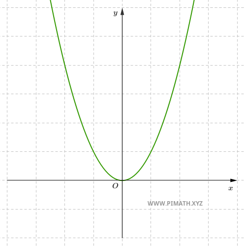
The graph of the monomial:
\[ y=x^2 \]
is a parabola with a vertical axis of symmetry:
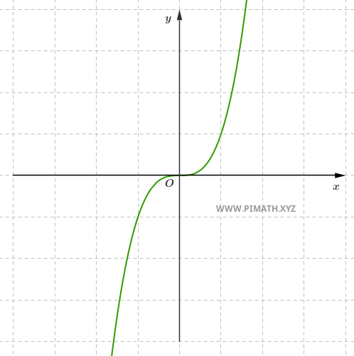
while:
\[ y=x^3 \]
produces a curve with point symmetry about the origin:
The overall behavior of a polynomial depends primarily on:
- its degree;
- the sign of the leading coefficient.
For instance, a polynomial of even degree with a positive leading coefficient tends to \(+\infty\) both as \(x\to +\infty\) and as \(x\to -\infty\).
Polynomials also form a particularly important class of functions because they are defined and continuous on the entire real line, with no discontinuities or singularities.